Computational Fluid Structure Interaction - Computational Hemodynamics: Theory, Modelling and Applications - page 120

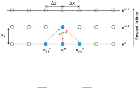
Fig. 5.23 Numerical approximation of the convection-diffusion equation onto discrete nodes. The
values on the new time step n +1 , are found from explicitly from values at the current time step n

∆
∆

t
x uuD

∆
∆

t
x

( )

n + 1 n n n n n n

u =− −+ −+ u A ( ) u 2 u u (5.43)

i i i + 1 i − 1 i + 1 i i − 1

2

2

This equation is looped over each node in a grid mesh. Schematically this is shown
in Fig. 5.23 , where the value of each node at the next time step n + 1 is given explic-
itly in terms of the values at the current time step n . Constant values for the problem
include:

A = 1 ∆ t = 0 005 . ∆ x = 005 .

D = 01 . n 200 = total x = 10 .

The solution is obtained by calculating Eq. (5.43) over every node. Since the solu-
tion solves for nodes at n + 1 based on nodes at time n , we need to provide an initial
condition for all nodes at time t = 0 to start the calculations. We set the flow do-
main with an initial sine wave velocity profile shown in Fig. 5.24 defined by

u xt ( , = =− 0) sin(2 π ) + 1 (5.44)

The solution over n = 150 time steps are shown in Fig. 5.25 where the solution is a
decaying travelling wave. The convection term transports the initial wave profile,
while the diffusion term dissipates it. We see that for Case B the initial velocity wave
dissipates rapidly due to the increased diffusion ( D = 0.3 for Case B compared with

Fig. 5.24 Initial velocity pro-
file applied onto the discrete
nodes in the 1D domain