Biomedical Engineering Reference
In-Depth Information
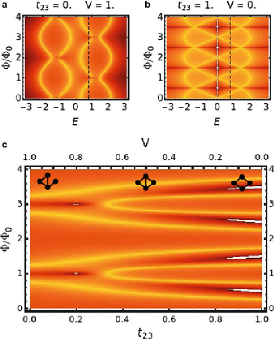
Fig. 8.6
Transmission function
T
13
(
E
,
Φ
)
for (
a
) the small orbit with
t
23
=
0and
V
=
1and(
b
)the
big orbit with
t
23
8 is shown by the
vertical dashed lines
in (
a
)and(
b
). The
left and right edges
of (
c
) correspond to the transmission
throughout the small and large orbits, respectively, as shown in the
insets
. The transition from one
to the other is performed by varying the interarm coupling along
V
=
1and
V
=
0. (
c
) Transmission
T
13
(
V
,
Φ
)
along the cut
E
=
0
.
t
23
.
Bright lines and dark
regions
represent zones of high and low transmission, respectively. The transmission
T
=
1
−
(
V
,
Φ
)
along
the left edge
(
V
=
1
)
shows a period of 2
Φ
0
while along the right edge (
V
=
0) has a period of
Φ
0
=
−
coupling between QD2 and QD3 (
t
23
) increases as
V
1
t
23
, shown in Fig.
8.6
c.
=
The transmission through the small orbit (Fig.
8.6
a), for
V
1, shows a period 2
Φ
0
=
in the flux. In the conductance through the large orbit (Fig.
8.6
b), for
V
0, the
period
0
becomes apparent. Finally, the bottom panel (c) shows the variation of
the transmission at
E
Φ
=
.
0
8 as a function of
V
and
Φ
. The smooth transition from
=
−
Fig.
8.6
a to b is realized by interpolating along
V
1
t
23
,insuchawaythatas
V
increases
t
23
decreases, and reciprocally.
As a final example consider the (1,2) configuration with the lead L attached to
QD1 and lead R connected to QD2. There are three interfering paths, namely, the