Biomedical Engineering Reference
In-Depth Information
a
b
1
1
0.8
0.8
0.6
0.6
0.4
0.4
0.2
0.2
0
0
0
0.2
0.4
0.6
0.8
1
0
0.2
0.4
0.6
0.8
1
F
F
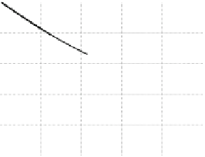
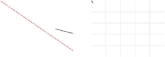
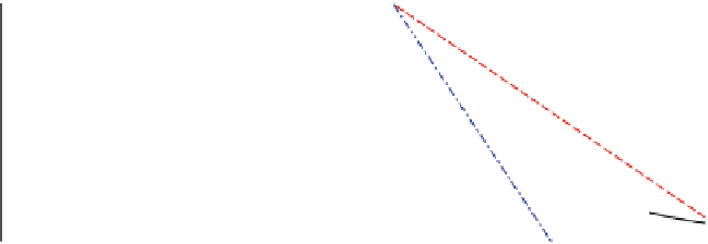
Fig. 6.2
(
a
) Normalized variation of the potential drop in the spontaneous potential
Δφ
sp
across a
cuboid-shaped QD as a function of the height to base length ratio
F
=
h
/
B
.
Solid line
shows
Δφ
sp
using the exact solution from [
38
];
dashed (red) line
is calculated using Eq. (
6.9
). (
b
)
Solid line
:
normalized variation of the strain-related piezoelectric potential
pz
using exact solution from
[
38
].
Dashed (red) and dashed-dotted (blue) lines
: results from Eq. (
6.10
) assuming, respectively,
constant strain only (first term), and allowing also for first-order changes in the strain field (both
terms). [From [
16
]]
Δφ
the QD compared to a QW. By using the equations given in [
38
], it can be shown that
the potential difference
Δφ
pz
between the center of the top and the bottom surfaces
of the QD varies for small
F
as [
16
]:
C
1
h
1
F
2
√
2
π
C
2
h
2
√
2
π
Δφ
pz
≈
−
−
F
,
(6.10)
with
2
ε
0
(
2
e
31
+(
1
−
A
)
e
33
)
C
1
=
,
(6.11)
ε
ε
r
0
and
C
2
=
ε
0
A
[
2
e
15
−
e
33
+
e
31
]
.
(6.12)
ε
r
ε
0
1
+
ν
=
Here,
ε
0
is the isotropic misfit strain,
ε
r
is the dielectric constant, and
A
,
1
−
ν
with
being the Poisson ratio. The first term on the right-hand side (RHS) of
Eq. (
6.10
) is of the same form as the result for the potential difference
ν
sp
arising
from the spontaneous part given by Eq. (
6.9
). The second (
C
2
) term originates from
the strain redistribution in the QD, including contributions from the shear strain part
of the piezoelectric polarization (
e
15
) as well as axial terms related to
e
31
and
e
33
,cf.
Eq. (
6.2
). In the case of a QW we have a biaxial compressive strain in the
c
-plane and
a tensile strain along the
Δφ
[
]
0001
-direction. Due to the finite dot size, a QD structure