Optimisation of Cancer Drug Treatments Using Cell Population Dynamics - Mathematical Methods and Models in Biomedicine - page 287

1

G1 sim
SG2M sim
G1 data
SG2M data

0.9

0.8

0.7

0.6

0.5

0.4

0.3

0.2

0.1

0

0 5 10 15 20 25 30

time (h)

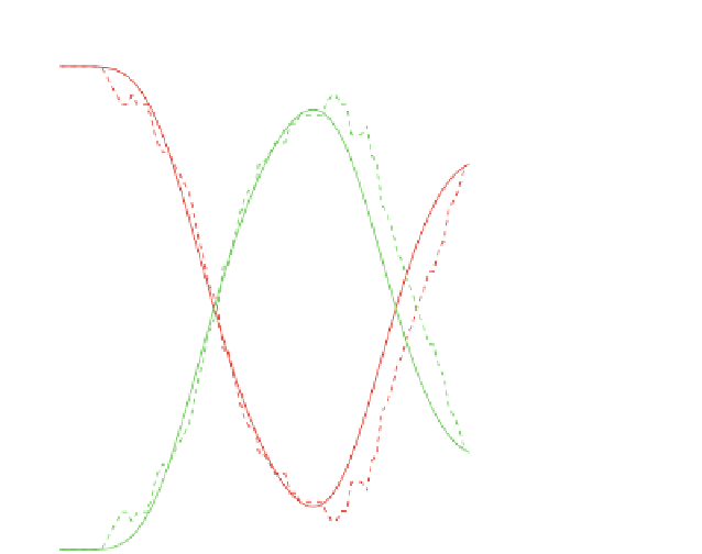
Fig. 2 M

( green or light grey ) from biological data ( dashed line ) and from numerical simulations ( solid line ).
Our model results in a reasonably good fit to biological data

Time evolution of the percentages of cells in the phases G 1 ( red or deep grey )and S / G 2 /

the random variable corresponding to the time spent in G 1 and S M .This

enabled us to determine the expression of the transitions rate according to the
formula ( 22 ). We then compared the solutions of the system with cell recordings
that had previously been synchronised “by hand”, i.e., all recordings were artificially
made to start simultaneously at the beginning of G 1 phase. The result is shown on
Fig. 2 . Note that using an inverse problem method—see Sect. 5 —instead of ours
could have consisted here in determining the parameters of the model, i.e., K i → i + 1
transition functions, by minimising an L 2 distance between this experimental data
curve and a theoretical, parameter-dependent curve representing these data.

/ G 2 /

7.5 Optimising Eigenvalues as Objective and Constraint

Functions

We then used combined time-independent data on phase transition functions,
obtained from experimental identification of the parameter functions K i → i + 1 ( t , x )=

κ i ( x ) in the uncontrolled model, with cosine-like functions representing the periodic