Data Assimilation in Brain Tumor Models - Mathematical Methods and Models in Biomedicine - page 248

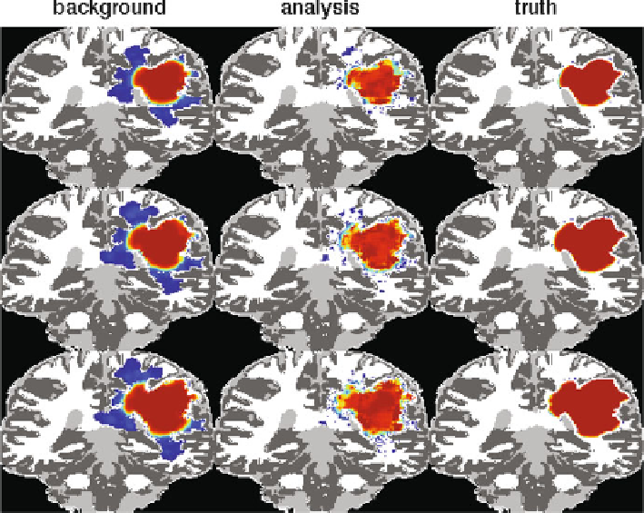
Fig. 7 Cell density plots for the second observing system simulation experiment where Eq. ( 66 )
is used to form the components of the observation operator. The first, second, and third rows
correspond to days 120, 150, and 180 of the experiment

α k is the logistic growth rate of the k th ensemble solution and ∂ u k ( x , t )
∂

where is the

t

time derivative of the growing cell density for the k th ensemble member. η ( x ) is as

in Eq. ( 65 ).
Figure 7 displays results of the experiment with Eq. ( 66 ) used to form the
components of the observation operator. The rows correspond to days 120, 150,
and 180 of the experiment. In this case assimilation of observations yields an
analysis that has invaded essentially the same area of the truth, but the tumor core
(region composed red grid points) is heterogenous and slightly smaller in overall
size. If we compare the analysis on day 120 to the background at day 150, we
see that the analysis grows to have about the same tumor core size as the truth
between data assimilation steps, but has a greater area of infiltration. Taking into
consideration that for the chosen parameter values, the ensemble mean is more
invasive than the truth and that the contrast enhancement for this case depends on
the time rate of change of the growing cells, we can think of the data assimilation
as having a “braking” effect that temporarily slows down the overall growth of the
ensemble mean.