Data Assimilation in Brain Tumor Models - Mathematical Methods and Models in Biomedicine - page 245

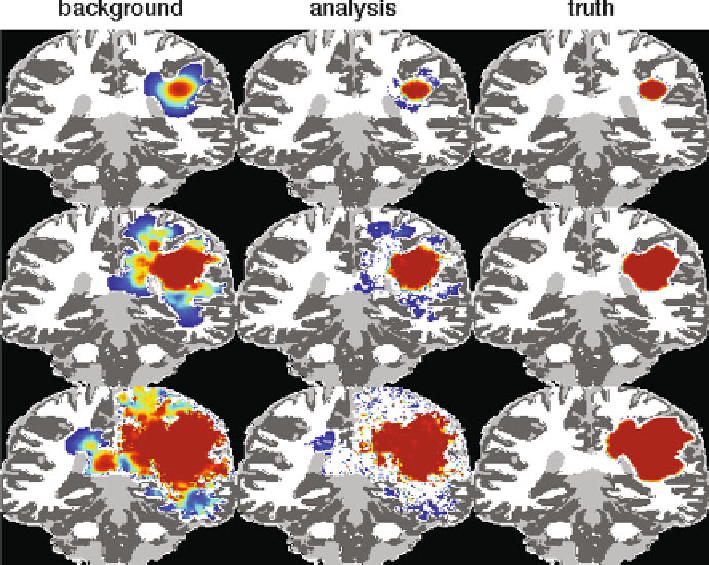
Fig. 4 Cell density plots for our first observing system simulation experiment. The first, second,
and third rows correspond to day 1, 90, and 180 of the experiment. See text for additional details

be the tumor cell
density for the k th ensemble member at location x and time t .Then

The value of H is computed pointwise as follows. Let u k ( x , t )

max 0 min 1

u k ( )

T max + η (

x , t

h k ( x )= , , x ) , (65)

η (

) [ − . , . ]

where and

T max is the carrying capacity for the k th ensemble solution. The value of h k (which is
confined to the unit interval) is the component of the H corresponding to the location
x in the brain domain. Note that the

x is a uniformly distributed random value in the interval 0 1 0 1

's are independent. The synthetic observations
are computed by applying H to the truth with the appropriate carrying capacity.
Figure 4 shows the results of our first experiment. The brain geometry is
displayed where the cell density is below 5 cells mm − 2 . The color coding is done on
a 128 color linear scaling analogous to a temperature plot where red corresponds to
cell densities at or near the carrying capacity of the truth and blue represents lower
cell densities. The first, second, and third rows correspond to days 1, 90, and 180
of the experiment. The left column, labeled “background,” shows the background
ensemble mean. The middle column, labeled “analysis,” shows the analysis mean.

η