Medical Imaging as a Bone Quality Determinant and Strength Indicator of the Femoral Neck - Biomedical Engineering Systems and Technologies - page 194

3.3 FEA Simulation

In order to associate the ultimate compression strength of the samples, to fragility
fracture risks of the femoral neck, the geometry of the specimens was reverse engi-
neered and employed in a linear elastic simulation of a gait type loading scenario
considering combined multiaxial forces [38].
During the simulation, the specimens were once again considered as a uniform-
isotropic material, comprising of cortical and cancellous bone tissue, to directly facili-
tate the correlation of the DXA measurements to the fracture risk of the femoral neck.
The experimentally determined mechanical properties were adopted as bulk properties
of the compound material and assigned as such in the simulation. The Poisson ratio
was assigned as 0,3 corresponding to a mean value of cortical and cancellous bone
[39,40] regardless DXA value.
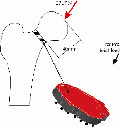
The acting loads on the femur, comprised of a 2317N joint force [41], evenly
distributed over the femoral head (inclined by 24 o to the frontal plane and 6 o to the
sagittal one). This force was remotely applied on the upper surface of the reverse
engineered specimens at a distance of 46mm corresponding to the mean distance from
the tip of the femoral head at which the specimens were severed from the femur. This,
based on the coordination system of the model, resulted in a vector force comprising
of F x = 689N, F y = 942N and F z = 2001N for axis x, y and z respectively.
The abductor muscle was considered as inactive, as this muscle force acts during
the lift up of the foot, thus loading the trochanter during the relaxation of the joint
force. As the abductor muscle force has been documented to amount to approximately
703N, the worst case scenario during normal loading of the femur, relates to the
aforementioned 2317N joint force.
The acting force and boundary conditions were chosen to mimic the average load-
ing history encountered during walking of an adult human, corresponding to 10.000
daily cycles [41] and are schematically represented in figure 5.

Fig. 5. Applied load and boundary conditions of the developed FEA model