Biomedical Engineering Reference
In-Depth Information
Frequency
(radians/s)
.001
.356
1.17
2.59
8.53
12.7
18.9
41.8
62.1
137
304
1000
20 log
j
G
j
6.02
6.02
5.96
5.74
3.65
1.85
0.571
6.64
9.95
16.8
23.6
34.0
(dB)
Phase
(degrees)
.086
3.06
10
22
64.9
88.14
116.0
196.0
259.0
479.0
959.0
2950.0
35.
Sinusoids of varying frequencies were applied to an open-loop system and the following
results were measured. Construct a Bode diagram and estimate the transfer function.
Frequency (radians/s)
0.11
0.24
0.53
1.17
2.6
5.7
12.7
28.1
62
137
304
453
672
1000
Magnitude Ratio,
j
G
j
2.0
2.0
2.0
2.0
1.93
1.74
1.24
0.67
0.32
0.15
.07
0.044
0.03
0.02
Phase (degrees)
0.62
1.37
3.03
6.7
14.5
29.8
51.8
70.4
80.9
85.8
88.1
88.7
89.7
89.4
36.
Sinusoids of varying frequencies were applied to an open-loop system and the following
results were measured. (Data from [43].) Construct a Bode diagram for the data.
Frequency
(radians/s)
1
3
7
10
15
20
25
30
35
40
50
60
70
80
90
100
110
120
130
140
Magnitude
Ratio,
1
.95
.77
.7
.67
.63
.6
.53
.48
.44
.35
.31
.33
.35
.32
.32
.3
.29
.27
.26
j
G
j
Phase
(radians)
.035
.227
.419
.541
.611
.768
.995
1.08
1.24
1.31
1.52
1.92
1.61
1.83
2.08
2.23
2.53
2.72
2.9
3.0
Estimate the transfer function if it consists of (a) two poles; (b) a pole and a complex pole
pair; (c) two poles, a zero, and a complex pole pair; (d) three poles, a zero, and a complex
pole pair. (Hint: It may be useful to solve this program using the MATLAB System
Identification toolbox or Seidel's program.)
37.
The following data were collected for the step response for an unknown first-order system.
Find the parameters that describe the model.
T
0.0
0.005
0.01
0.015
0.02
0.025
0.03
0.035
0.04
0.045
0.05
0.055
0.06
0.1
0.00 3.41 5.65 7.13 8.11 8.75 9.18 9.46 9.64 9.76 9.84 9.90 9.93 10.0
38.
Suppose a second-order underdamped system response to a step is given by Eq. (13.73) and
has
v(t)
10.1. Find z and o
n
. A stylized 10
saccade is shown in the
following figure. Estimate z and o
n
for the Westheimer model. Calculate the time to peak
velocity and peak velocity.
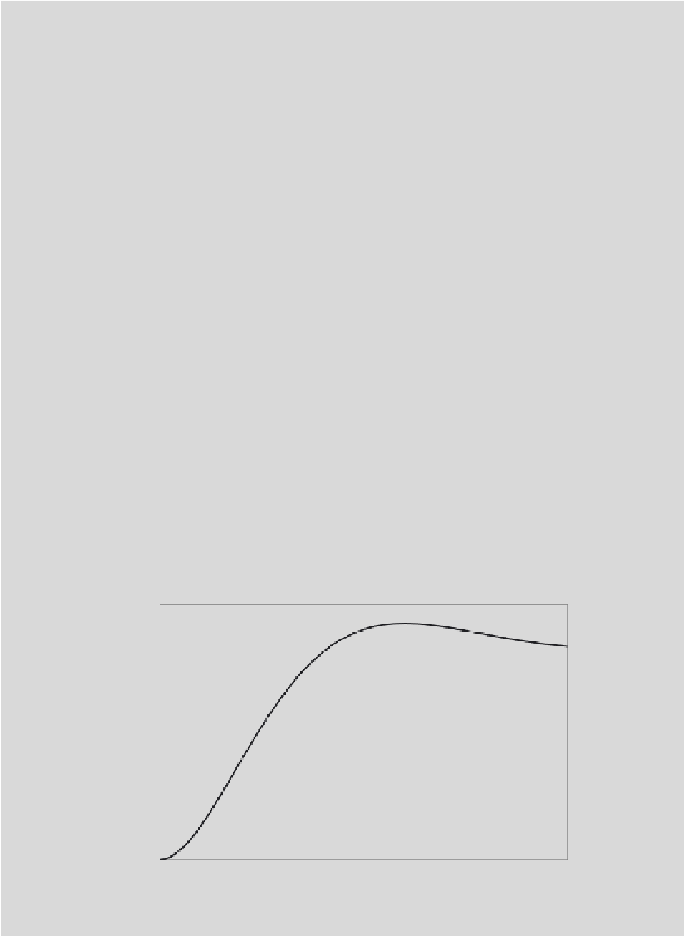
39.
Consider the data in Figure 13.80. Estimate z
,
o
n
, and f if the system has the solution of the
form of Eq. (13.73).
C
¼
10,
T
p
¼
0.050, and
y(T
p
)
¼
12
10
8
6
4
2
0
0
0.01
0.02
0.03
0.04
0.05
0.06
0.07
Time (s)
FIGURE 13.80
Illustration for Exercise 39.