Biomedical Engineering Reference
In-Depth Information
Slab
Cylinder
Sphere
C
0
C
0
C
0
C
0
C
0
r
x
r
R
s
x = 0
x = L
x = 0
r = R
c
(a)
(b)
(c)
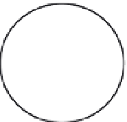
FIGURE 6.24
The three possible configurations considered by the mass transfer equations.
Reproduced from [12].
The manner in which the distance variables are defined in each case is shown in
Figure 6.24. A standard technique in the analysis of differential equations describing
transport phenomena is to scale the variables so they are dimensionless and range in
value from 0 to 1. This allows the relative magnitude of the various terms of the equations
to be evaluated easily and allows the solutions to be plotted in a set of graphs as a
function of variables that are universally applicable. For all geometries,
C
is scaled by
C
¼
C
=
C
o
its maximum value,
C
o
—that is,
. Distance is scaled with the diffusion path
x
¼
x
=
L
r
¼
r
=
R
c
length, so for a slab,
.Withthese
definitions, the boundary conditions for all three geometries are no flux of nutrient at the
center
; for a cylinder,
;andforasphere,
r
¼
r
=
R
s
0) and that
C
¼
ð
dc
=
dx
dc
=
dr
¼
at x
r
x
r
1).
The use of scaling allows the solutions for all three geometries to collapse to a common
form:
,
0
,
,
¼
1atthesurface(
,
,
¼
f
2
C
¼
1
x
2
2
ð
1
Þ
2
,
which is often called the Thiele modulus. The Thiele modulus represents the relative rates
of reaction and diffusion and is defined slightly differently for each geometry:
All of the system parameters are lumped together in the dimensionless parameter
f
2
2
2
2
slab
¼
Q
i
=
L
cylinder
¼
Q
i
=
Rc
sphere
¼
Q
i
=ð
L
¼ð
R
=
3
Þ
Þ
f
2
f
2
f
2
,
,
C
o
D
t
C
o
D
t
C
o
D
t