Biomedical Engineering Reference
In-Depth Information
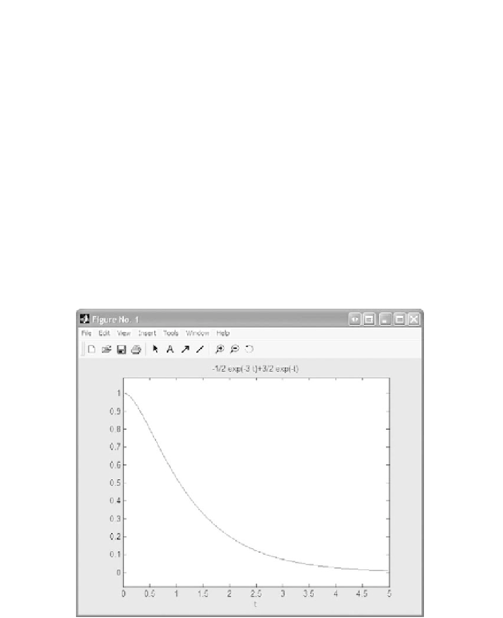
To plot these results, we use the MATLAB plotting function called “ezplot”, an easy way to
plot functions defined by symbolic functions. To plot the previous result, we execute
>>
ezplot(y, [0, 5])
which gives the results shown in Figure A.6.
The argument enclosed in the brackets of the “ezplot” command is the initial and final
points.
If the initial conditions are not entered in the “dsolve” command, the solution is calcu-
lated in terms of unknown coefficients. To illustrate, consider entering the command
“dsolve” without initial conditions,
>>
dsolve('D2y
þ
4
*
Dy
þ
3
*
y
¼
0')
which gives us
C1
*
exp (
t
Þþ
C2
*
exp (
3
*
t
Þ
The values for C1 and C2 are determined from the initial conditions.
To solve
10
8
10
8
y
þ
16, 000
y
þ
y
¼
5
t
FIGURE A.6
An illustration of the MATLAB plotting function, “ezplot.”