Biomedical Engineering Reference
In-Depth Information
210
p
e
2
t
sin(
p
t
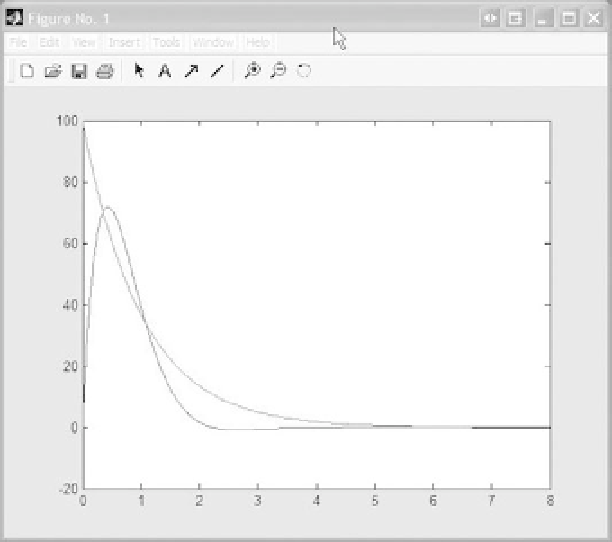
FIGURE A.4
The functions
e
t
and
f
¼
100
y
¼
) graphed using the MATLAB “plot”
command.
Before exporting the data, it is easiest to collect the data in a single matrix with the inde-
pendent variable listed first, along with the dependent variables—each evaluated at the
points listed for the independent variable. Consider exporting the function shown in
Figure A.3, where
t
and
y
are given by
>>
t
¼
linspace(0, 8, 1000);
>>
y
¼
297
*
sin (1.414
*
t).
*
exp (
2
*
t);
1000 row vectors, so we must take the trans-
pose of each row vector when concatenating to form the new matrix
Keep in mind that
t
and
y
are stored as 1
data
by
[t
0
,y
0
];
>>
data
¼
2. If there are additional vectors to be
exported as in Figure A.4, we concatenate all the data with the command “data
Data is stored in the matrix
data
with order 1000
[t
0
,y
0
,f
0
];”.
To export the data to an arbitrary ASCII file “output.txt”, with tabs separating each vari-
able, we use the following command:
¼
>>
save output.txt data - ascii - tabs
This file is stored in the MATLAB subfolder “work” by default. Next, open the file
“output.txt” in Excel. At this time, the data are stored in the first two columns in the work-
space. From here one can use the step-by-step “chart wizard” to create a “scatter chart” like
that shown in Figure A.5.