Biomedical Engineering Reference
In-Depth Information
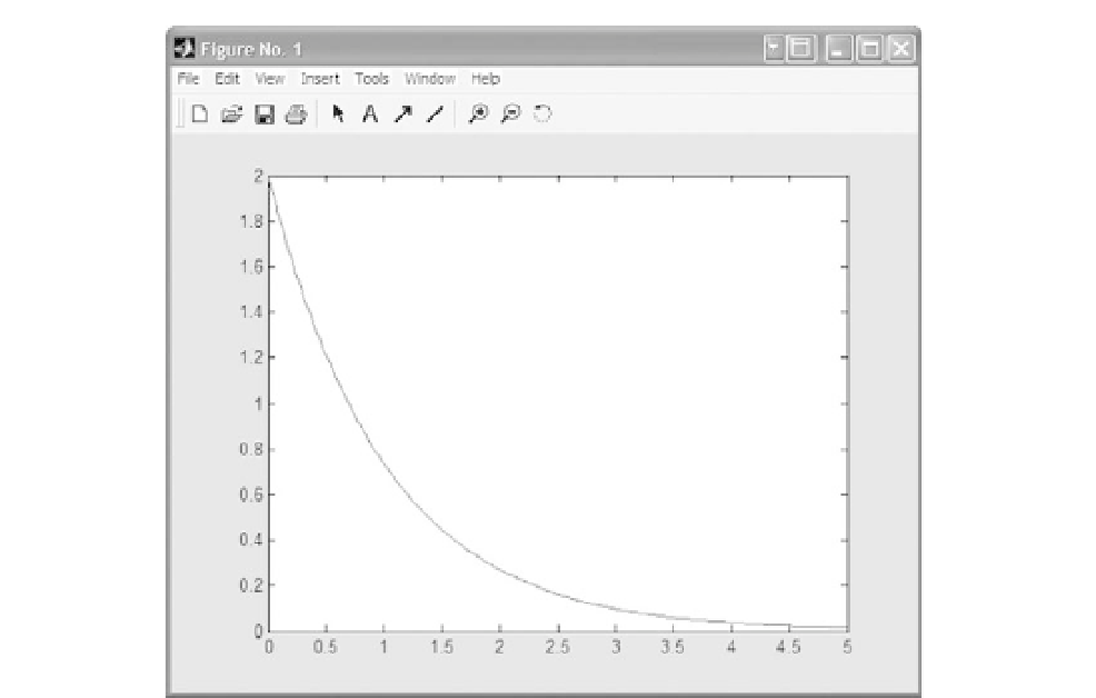
FIGURE A.2
MATLAB plot of the function
f
¼ 2
e
t
plotted using the command fplot.
plot
Another plotting command is “plot(t,y)”, which plots
y
versus
t
with points connected by
straight lines. The independent variable
t
is easily defined using the “linspace” command
with the syntax “t
¼
linspace(a,b,n)” that generates a row vector of
n
linearly spaced ele-
ments over the timespan
.
For example, we can plot the function
a
to
b
210
p
e
2
t
p
t
y
¼
sin (
) using the following
commands:
>>
t
¼
linspace(0, 8, 1000);
>>
y
¼
297
*
sin(1.414
*
t).
*
exp (
2
*
t);
>>
plot(t, y)
The first command creates a 1000-element row vector
t
, with values ranging from 0 to 8.
The second command creates a 1000-element row vector
y
by multiplying sin (1.414
*
t) by
exp (
2
*
t) with the “.
*
” operation. The “.
*
” operation is the dot multiplication function
that performs an element-by-element multiplication. MATLAB generates an error if one
uses “
*
” instead of “.
*
” in the previous calculation, because it associates
t
as a 1
1000
row vector, which forces sin (1.414
*
t) as a 1
1000 row vector. In this case, the matrix multiplication is not valid because the order of
the matrices does not agree. The command “plot” graphs the function
1000 row vector and exp (
2
*
t) as a 1
y
in the time interval
from 0 to 8 with 1000 connected points as shown in Figure A.3.