Biomedical Engineering Reference
In-Depth Information
0.55
0.50
0.45
P
= 0.15 kN
P
= 0.10 kN
P
= 0.05 kN
P
= 0.0
0.40
0.35
0.30
0.25
0.20
0.15
0.10
0.05
0.00
-200
0
200
400
600
800
1000
1200
1400
1600
t
(day)
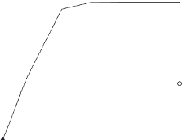
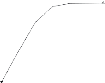
FIGURE 5.5
Variation of porosity
p
in the disuse-mode case.
below a certain (or critical) level. Here we define the value as 50%.
When the porosity approaches this value, biological factors will
stimulate the osteocytes to excrete more growth factors to resist the
loss of bone mass. This is clearly shown in Figure 5.5. It can also be
shown that when the loading vanishes, the velocity of bone remod-
eling is not as fast as in bone materials subjected to compressive
loads. This can be attributed to the lack of environmental stimuli,
resulting in a reduction of osteoclasts. Then fewer osteocytes are
resorbed and fewer growth factors are released, slowing down the
loss of bone mass.
• Case 3:
P
= 1.0 kN,
E
i
= 1, 10, 50, 100 V/m,
f
e
= 15 Hz. Figure 5.6 shows
the effect of electrical loading on the bone modeling process. It
can be seen that when environmental stimuli are insufficient, the
remodeling state of bone tissue will remain unchanged. As the elec-
trical loading increases to a particular level, bone modeling can be
triggered. A more intense electrical field can produce a less porous
and denser bone structure. But when the electrical loading is suf-
ficiently high, a further increase will have very little effect on the
bone modeling process. This is also due to an insufficiency of osteo-
clasts. The capacity of the body to produce osteoclasts restricts the
upper limit of growth factors. So the electrical loading that can effec-
tively stimulate bone modeling must have both an upper and a lower
limit. However, all these conclusions are based on the hypothetical
model. At this stage, we cannot give the exact values of these thresh-
olds, which require further experimental investigation in this field.