Biomedical Engineering Reference
In-Depth Information
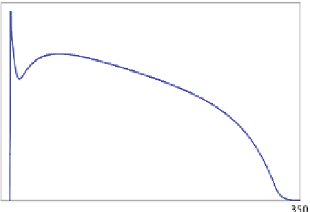
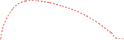
Fig. 14.3
Time evolution of
the electric fields in a specific
epicardial position of the
tissue. Plotted quantities are
the transmembrane potential
v
, gate variables
w
=
(w
1
,w
2
,w
3
)
and the
mechanical activation
γ
f
which are all presented in
dimensionless form
385 kPa, has shown
to yield a qualitatively correct end-systolic displacement magnitude (around 25 %)
and rotation of the left ventricle, as reported in Rossi et al. (
2012
). Quadratic finite
elements are used for displacement, whereas all other fields are discretized using
continuous piecewise trilinear elements, in order to satisfy Brezzi-Babuška
inf-sup
condition. The timestep, fixed during the simulation, is
t
Robin boundary condition
m
u
+
Pn
=
0
, with
m
=
μ
=
0
.
01 ms and, as usual
in electromechanically coupled computational models (see, e.g., Nash and Panfilov,
2004
; Cherubini et al.,
2008
; Pathmanathan and Whiteley,
2009
; Land et al.,
2012
),
we iterate between electrical and mechanical problems in a segregated mode. The
nonlinear equations arising from the discretization of the mechanical problem are
linearized using the Newton-Raphson method. We find that no more than 6 iterations
are needed to converge with a tolerance of
ε
tol
=
=
10
−
8
, with the maximum number
of iterations being always attained around the upstroke phase. The linear systems
are solved using the GMRES iterative method (with a tolerance of
10
−
7
).
The average overall CPU time spent per time step is 3
.
5 seconds, using 32 cores
distributed on 4 nodes on the Intel Harpertown cluster
Callisto
at EPFL.
1
An external stimulus
I
app
=−
ˆ
ε
tol
=
0, in order
to generate a traveling wave for the transmembrane potential, initially everywhere
at rest (
v
100 µA is applied at the apex at
t
=
84 mV). Figure
14.4
presents three snapshots of the solution of the
excitation-contraction problem at times
t
=−
540 ms,
where fiber directions are represented by the gray volume arrows and the color-map
shows the values of the transmembrane potential
v
on the undeformed solid. Notice
that the activation patterns adopt a profile dictated by the tissue anisotropy.
=
1,
t
=
40,
t
=
230 and
t
=