Biomedical Engineering Reference
In-Depth Information
Figure 2.4-10 Four different signals (left side) and their autocorrelation functions (right side). A: A truncated sinusoid. The reduction in
amplitude is due to the finite length of the signal. A true (i.e., infinite) sinusoid would have a nondiminishing cosine wave as its auto-
correlation function. B: A slowly varying signal. C: A rapidly varying signal. D: A random signal.
between standard correlation and covariance given in the
last section. Covariance and correlation functions are the
same except that, in covariance, the means have been
removed from the input signals,
x
(
t
) and
y
(
t
) [or just
x
(
t
)
in the case of autocovariance]:
ð
T
Auto
cov
ariance
h
C
xx
ð
s
Þ¼
1
T
½xðtÞxðtÞ
0
½xðt þ
s
ÞxðtÞdt
N
X
N
C
xx
½i¼
1
½xðkÞx½xðk þ iÞx
[Eq. 2.4.36]
k¼
1
ð
T
Cross
cov
ariance
h
C
xy
ð
s
Þ¼
1
T
½yðtÞyðtÞ
0
½xðt þ
s
ÞxðtÞdt
N
X
N
Cross
cov
ariance
h
C
xy½i
¼
1
½yðkÞyðkÞ
k¼
1
½xðk þ iÞxðkÞ
[Eq. 2.4.37]
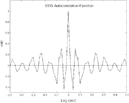
Figure 2.4-11 Autocorrelation function of the electroencephalo-
gram signal in
Figure 2.4-4
. The autocorrelation function
decorrelates rapidly probably due to the noise in the signal. Some
correlation is seen out to 0.5 seconds.
The autocovariance function can be thought of as
measuring the memory or self-similarity of the
deviation
of a signal about its mean level. Similarly, the