Basic signal processing - Biomedical Engineering Desk Reference - page 89

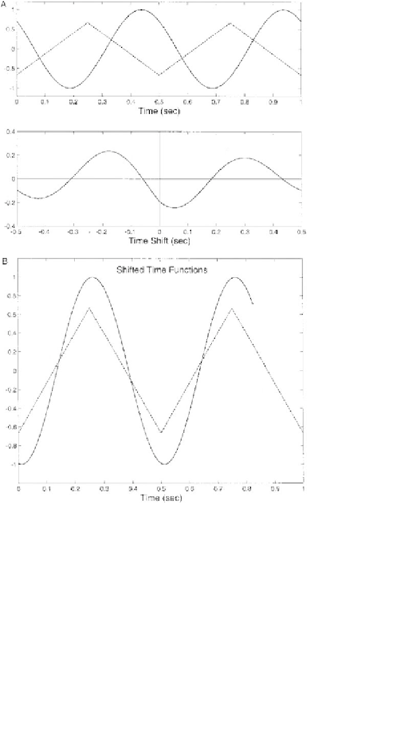
Figure 2.4-9 A(upper plot): a sinusoid and triangular wave at the same frequency, but not the same phase. Lower plot: The cross-correlation
function for these two waveforms shows a peak at around 0.18 seconds when the functions are most alike. B: The two functions in A
(upper plot) after shifting the sinusoid by an amount corresponding to the maximum cross-correlation given in A (lower plot).

function is involved in autocorrelation, the normalization
equation given in Eq. 2.4.29 reduces to 1/s 2 .)
Figure 2.4-11 shows the autocorrelation function of
the EEG signal shown previously. The signal decorrelates
quickly, reaching a value of zero correlation after a time
shift of approximately 0.03 seconds. However, the EEG
signal is likely to be contaminated with noise and the au-
tocorrelation function of a signal plus noise is the sum of
the autocorrelation function of the signal plus the auto-
correlation of the noise. Because noise decorrelates in-
stantly ( Figure 2.4-10D ), some of the rapid decorrelation

seen in Figure 2.4-11 is due to the noise. A common ap-
proach to estimating the autocorrelation of the signal
without the noise is to draw a smooth curve across the
peaks and use that curve as the estimated autocorrelation
function of signal without noise. From Figure 2.4-11 ,we
see that such an estimated function would decorrelate at
a longer time shift of 0.5 to 0.6 seconds.
Two operations closely related to autocorrelation
and cross-correlation are autocovariance and
cross-covariance. The relationship between correlation
and covariance functions is similar to the relationship