Basic signal processing - Biomedical Engineering Desk Reference - page 86

two signals, x ( t ) and y ( t ), over a time frame T is as
follows:

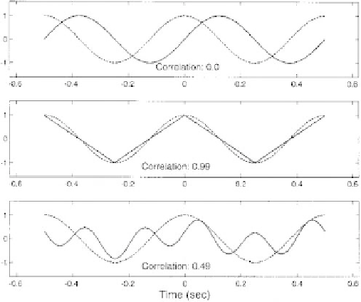
canceled by negative correlation over the rest of the
cycle. Mathematically, this is a demonstration that a sine
and a cosine of the same frequency are orthogonal func-
tions, which, by definition, are uncorrelated. Indeed,
a good way to test if two functions are orthogonal is to
assess their correlation. Correlation does not necessarily
measure general similarity, so a sine and a cosine of the
same frequency are, by this mathematical definition, as
unalike as possible, even though they have very similar
oscillatory patterns.

ð T

Corr ¼ 1
T

xðtÞyðtÞdt

0

or in discrete form
Corr ¼ 1

N X

N

xðkÞyðkÞ

[Eq. 2.4.28]

k ¼ 1

The integration (or summation in the discrete form) and
scaling (dividing by T or N ) simply take the average of the
product. It is common to modify Eq. 2.4.28 by dividing
by the square root of the product of the variances of the
two signals. This will make the correlation value equal to
1.0 when the two signals are identical and 1 if they are
exact opposites:

Example 2.4.6: Use Eq. 2.4.28 (continuous form) to find
the correlation (unnormalized) between the sine wave
and the square wave shown below. Both have an amplitude
of 1.0 V (peak-to-peak) and a period of 1.0 second.

Corr
s 1 s 2

Corr normalized ¼ q [Eq. 2.4.29]

where the variances, s 2 , are defined in Eq. 2.4.17 and Eq.
2.4.18 . The term correlation implies this normalization.
Correlation between two signals is illustrated in
Figure 2.4-7 , which shows various pairs of waveforms
and the correlation between them. Note that a sine and
a cosine have no (zero) correlation even though the two
are alike in the sense that they are both sinusoids (upper
plot). Intuitively, we see that this is because any positive
correlation between them over one portion of a cycle is

Solution: By symmetry, the correlation in the second half
of the 1-second period equals the correlation in the first
half, so it is only necessary to calculate the correlation
period in the first half period.

ð T

Corr ¼ 1
T

xðtÞyðtÞdt

0

ð T= 2

ð 1 Þ sin 2p t
T

dt

¼ 2
T

0

cos 2p t
T

T = 2

¼ 2
T

T
2p

0

Corr ¼ 1

p ð cos ð p Þð cos ð 0 ÞÞÞ ¼ 2 p

Covariance computes the variance that is shared between
two (or more) signals. Covariance is usually defined in
discrete format as follows:

Figure 2.4-7 Three pairs of signals and the correlation between
them as given by Equation 2.4.28 and normalized as in Equation
2.4.29 . Note the high correlation between the sine and triangle
wave (center plot) correctly expressing the general similarity
between them. However, the correlation between a sine and
cosine (upper plot) is zero, even though they are both sinusoids.

N 1 X

k

1

s xy ¼ ðx k xÞðy k yÞ [Eq. 2.4.30]

k¼ 1