Properties of materials - Biomedical Engineering Desk Reference - page 115

first objective in setting up an FEA problem is to identify
and specify the equations that define the behavior of un-
known variables in the continuum. Such equations typi-
cally result fromapplying the universal laws of conservation
of mass, momentum, and energy, as well as the constitutive
equations that define the stress-strain or other relation-
ships within the material. The resulting differential or in-
tegral equations must then be closed by specifying the
appropriate boundary conditions.
A ''well-behaved'' solution to the continuum problem
is guaranteed if the differential or integral equations and
boundary conditions systems are ''well posed.'' This
means that a solution to the continuum problem should
exist, be unique, and only change by a small amount
when the input data change by a small amount. Under
these circumstances the numerical solution is guaranteed
to converge to the true solution. Proving in advance that
a general continuum problem is ''well posed'' is not
a trivial exercise. Fortunately, consistency and conver-
gence of the numerical solution can usually be monitored
by other means, for example, the already mentioned
''patch test'' ( Zienkiewicz and Taylor, 1994 ).
The equations governing the description of a contin-
uum can be formulated via a differential or variational
approach. In the former, differential equations are used
to describe the problem; in the latter, integral equations
are used. In some cases, both formulations can be applied
to a problem. As an illustration we present a case for
which both formulations apply and later show that these
lead to the same FE equations.

V 2 u þ qu ¼ f in U (3.1.3.1a)

subject to the boundary conditions

u ¼ g on G 1 (3.1.3.1b)

vu
vn ¼ 0on G 2

(3.1.3.1c)

where V 2 h v 2 / v x 2 þ v 2 / v y 2 is the Laplacian operator in

two dimensions, n is the unit outward normal to the
boundary, and q, f, g are assumed to be constants for
simplicity, with q 0. Here, the boundary G is made up
of two parts, G 1 and G 2 , where different boundary
conditions apply.
When f ¼ 0, Eq. 3.1.3.1a means that the spatial change
of the gradient of u at any point in the xy space is
proportional to u . The boundary condition 1b sets u to
have a fixed value at one part of the boundary. On another
part of the boundary, the rate of change of u in the normal
direction is set to zero (boundary condition 3.1.3.1c).
The system represented by Eqs. 3.1.3.1a-c can be used
to describe the transverse deflection of a membrane,
torsion in a shaft, potential flows, steady-state heat
conduction, or groundwater flow ( Desai, 1979 ; Zien-
kiewicz and Taylor, 1994 ).

The variational formulation

A variational equation can arise, for example, from the
physical requirement that the total potential energy
(TPE) of a mechanical system must be a minimum. Thus
the TPE will be a function of a displacement function,
for example, itself a function of spatial variables. A
''function of a function'' is referred to as a functional.
We consider, as an example, the functional I (y)of
the function y( x , y ) of the spatial variables x and y , de-
fined by:
Ið y Þ¼ ðð

The differential formulation

Consider the function u ( x , y), defined in some two-
dimensional domain U bounded by the curve G
( Fig. 3.1.3-4 ), which satisfies the differential equation

Γ 1

n ðV y Þ 2 þ q y 2 2y f o dU

(3.1.3.2)

U

h

Ω

( Strang and Fix, 1973 ; Zienkiewicz andTaylor, 1994 ). The
relevant question is that of all the possible functions y( x ,
y ) that satisfy Eq. 3.1.3.2 , what particular y( x , y ) mini-
mizes I (y)? We get the answer by equating the first varia-
tion of I (y), written dI(y), to zero. To performthe variation
of a functional, one uses the standard rules of differenti-
ation. It can be shown that the variation of I (y) over y
results in Eq. 3.1.3.1a , provided Eqs. 3.1.3.1b and
3.1.3.1c hold and the variation of y is zero on G 1 . Thus the
function that minimizes the functional defined in
Eq. 3.1.3.2 is the same function that solves the boundary
value problem given by Eqs. 3.1.3.1a-c .

Γ 2

A B

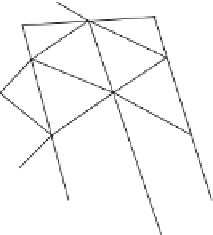
Fig. 3.1.3-4 (A) A continuum U enclosed by the boundary
G ¼ G 1 U G 2 ; the function itself is specified on G 1 and its derivative
on G 2 . (B) A finite element representation of the continuum. The
domain has been discretized with general arbitrary triangles of size
h, with the possibility of having curved sides.