Biomedical Engineering Reference
In-Depth Information
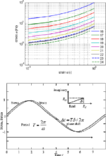
Fig. 6.10
The stress-strain
curves for a ladder network
model of the level 24,
building up additional cells,
until level 16
Fig. 6.11
Example of stress
and strain as a function of
time with normalized units.
Observe the phase shift
6.3.2 Sinusoidal Variations of Strain
In the previous section, a stepwise strain excitation was applied in steps of 10 % until
100 %. Similarly to the calculus presented previously, the new fractal-mechanical
model can be excited by a dynamic strain excitation; i.e. a sinusoidal excitation,
which is closer to the breathing phenomenon. It is noteworthy to realize that since
our model consists of a combination of springs and dampers, the stress-strain curve
will be a result of the two individual curves from Fig.
6.1
. Moreover, since we
only characterize the respiratory zone by the viscoelastic lung parenchyma, we also
expect a stress-strain curve as in Fig.
6.2
.
Oscillatory stress and strain histories are represented by sinusoid functions. Sup-
posewehave
σ(ωt)
σ
0
sin
πt
, in which
t
denotes time,
σ
0
denotes the amplitude,
and
ω
is the angular frequency. The sine function repeats every 2
π
radians. So
σ(ωt
=
σ(ωt)
. The time
T
required for the sine function to complete one
cycle is obtained from
ωT
+
2
π)
=
=
=
2
π/ω
. In a viscoelastic material, stress
and strain sinusoids are out of phase. To represent the phase shift consider two sinu-
soids, sin
ωt
and sin
(ωt
+
δ)
. The quantity
δ
is called the phase angle. In a plot of
the two waveforms, the sinusoids are shifted with respect to each other on the time
axis as in Fig.
6.11
. Recall that the cosine function is
π
/2 radians out of phase with
2
π
,or
T