Biomedical Engineering Reference
In-Depth Information
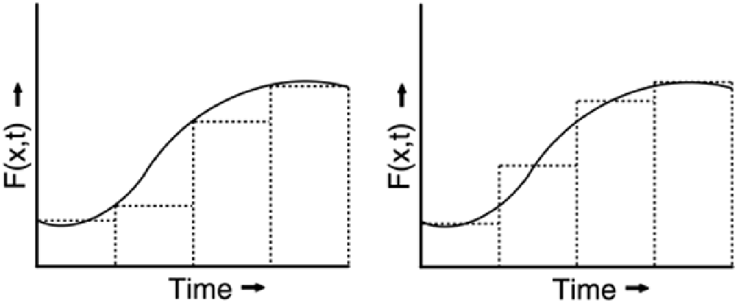
Figure 9-6. Euler (left) versus Runge-Kutta (right) Integration Methods.
The Euler method is simpler to implement, but the Runge-Kutta method is
more accurate and more efficient.
Two of the most popular integration methods are the Euler and Runge-Kutta methods. The Euler
method is simple to implement but the least elegant, with truncation errors inversely proportional to
step size and round-off errors directly proportional to step size. A larger step size or time slice results
in fewer round-off errors, which are cumulative, at the expense of increased truncation errors. In
addition, because the Euler method ignores the underlying change in the equation, it becomes
unstable with a relatively large step size.
The Runge-Kutta method of numerical integration is more elegant, more efficient, more stable, and
more accurate than the Euler method. The basic Runge-Kutta method allows the use of a larger step
size for a given round-off error, and so reduces computational time, even though the algorithm is
more complex than that of the Euler method. A variation of the basic Runge-Kutta method, the
Adaptive Runge-Kutta method, adjusts step size dynamically during program execution to reflect the
rate of change in the equation. For example, it decreases step size with an increasing rate of change
in the equation, and increases step size when the rate of change diminishes. As a result, while the
Euler method might require 1,000 steps to evaluate an equation, the Runge-Kutta method might
involve only 100 steps.
As illustrated in
Figure 9-6
, the Euler method of numerical integration involves repeatedly
accumulating slices of area, of constant width, to determine the area under the curve defined by the
differential equation. In contrast, the Runge-Kutta method considers the slope of the equation at
multiple points along each time slice, resulting is better curve fit and less truncation error.
Random Numbers
Random numbers from a variety of distributions form the basis of many simulation techniques. At
best, most digital methods produce nearly random numbers, typically through programs called
pseudorandom number generators.
Figure 9-7
shows that the output from the pseudorandom
generator of a popular simulation package running under Windows on a Pentium III hardware
platform isn't perfect. Ideally, the numbers would be evenly distributed throughout the range, with
no significant peaks and no holes, such as the band of missing numbers around 22,000.
Figure 9-7. Frequency Plot of a Pseudorandom Number Generator. The plot
represents the cumulative output of 20,000,000 iterations of the generator