Cryptography Reference
In-Depth Information
From the point of view of complexity, the Viterbi algorithm requires the
calculation of
2
ν
+1
accumulated metrics at each instant i and its complexity
varies linearly with the length of sequence
k
or of decoding window
l
.
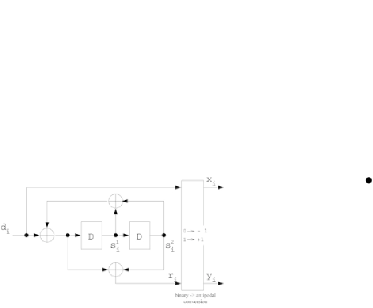
Example of applying the Viterbi algorithm
Let us illustrate the different steps of the Viterbi algorithm described above by
applying it to decode the binary recursive systematic convolutional code (7,5)
with 4 states and encoding rate
R
=1
/
2
(
m
=
n
=1
). The structure of the
encoder and the trellis are shown in Figure 5.20.
s
s
i
i
1
(1, 1)
(00)
(+1, +1)
(+1, +1)
(01)
(1, 1)
(+1, 1)
(10)
(1, +1)
(1, +1)
(+1, 1)
(11)
(x
i
, y
i
(x
i
, y
i
)
)
d
i
d
i
=0
=1
Figure 5.20 - Structure of the recursive systematic convolutional code (7,5) and asso-
ciated trellis.
Calculate the branch metrics at instant
i
:
d
(
T
(
i,
0
,
0
)) =
d
(
T
(
i,
1
,
2
)) =
(
X
i
+1
)
2
+
(
Y
i
+1
)
2
d
(
T
(
i,
0
,
2
)) =
d
(
T
(
i,
1
,
0
)) =
(
X
i
−
1
)
2
+
(
Y
i
−
1
)
2
1
)
2
+
(
Y
i
+1
)
2
d
(
T
(
i,
2
,
3
)) =
d
(
T
(
i,
3
,
1
)) =
(
X
i
+1
)
2
+
(
Y
i
−
d
(
T
(
i,
2
,
1
)) =
d
(
T
(
i,
3
,
3
)) =
(
X
i
−
1
)
2
Calculate the accumulated metrics of the branches at instant
i
:
1
,
0
)+(
X
i
+1)
2
+(
X
i
+1)
2
λ
(
T
(
i,
0
,
0
)) =
μ
(
i
−
1
,
0
)+
d
(
T
(
i,
0
,
0
)) =
μ
(
i
−
1
,
1
)+(
X
i
+1)
2
+(
X
i
+1)
2
λ
(
T
(
i,
1
,
2
)) =
μ
(
i
−
1
,
1
)+
d
(
T
(
i,
1
,
2
)) =
μ
(
i
−
1)
2
+(
X
i
−
1)
2
λ
(
T
(
i,
0
,
2
)) =
μ
(
i
−
1
,
0
)+
d
(
T
(
i,
0
,
2
)) =
μ
(
i
−
1
,
0
)+(
X
i
−
1)
2
+(
X
i
−
1)
2
λ
(
T
(
i,
1
,
0
)) =
μ
(
i
−
1
,
1
)+
d
(
T
(
i,
1
,
0
)) =
μ
(
i
−
1
,
1
)+(
X
i
−
1)
2
+(
X
i
+1)
2
λ
(
T
(
i,
2
,
1
)) =
μ
(
i
−
1
,
2
)+
d
(
T
(
i,
2
,
1
)) =
μ
(
i
−
1
,
2
)+(
X
i
−
1)
2
+(
X
i
+1)
2
λ
(
T
(
i,
3
,
3
)) =
μ
(
i
−
1
,
3
)+
d
(
T
(
i,
3
,
3
)) =
μ
(
i
−
1
,
3
)+(
X
i
−
1
,
2
)+(
X
i
+1)
2
+(
X
i
−
1)
2
λ
(
T
(
i,
2
,
3
)) =
μ
(
i
−
1
,
2
)+
d
(
T
(
i,
2
,
3
)) =
μ
(
i
−
1
,
3
)+(
X
i
+1)
2
+(
X
i
−
1)
2
λ
(
T
(
i,
3
,
1
)) =
μ
(
i
−
1
,
3
)+
d
(
T
(
i,
3
,
1
)) =
μ
(
i
−