Graphics Reference
In-Depth Information
a
b
B
0
B
1
B
2
Current block
Co-located block
C
1
C
0
A
1
A
0
Fig. 5.4
Motion vector predictor and merge candidates. (
a
) Temporal. (
b
) Spatial
A0, A1
B0, B1, B2
available?
available?
yes
yes
first
non-scaled
MV found
first
non-scaled
MV found
not
found
not
found
find
non-
scaled MV
find
non-
scaled MV
no
yes
no
A0 or A1
available?
A0 or A1
available?
find
scaled MV
with
both curr. ref pic and ref pic
being short term ref pics
Find
non-scaled MV
or
scaled MV
with
both curr. ref pic and
ref pic being
short term ref pics
Find
non-scaled MV
or
scaled MV
with
both curr. ref pic and
ref pic being
short term ref pics
first scaled
MV found
first non-scaled
or scaled MV
found
first non-scaled
or scaled MV
found
A
B
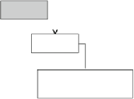
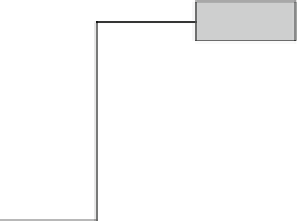
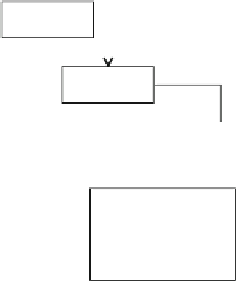
Fig. 5.5
Derivation of spatial AMVP candidates A and B from motion data of neighboring blocks
A0,A1,B0,B1andB2
motion vectors need to be scaled according to the temporal distances between
the candidate reference picture and the current reference picture. Equation (
5.3
)
shows how the candidate motion vector
mv
cand
is scaled according to a scale factor.
ScaleFactor is calculated in Eq. (
5.4
) based on the temporal distance between the
current picture and the reference picture of the candidate block td and the temporal
distance between the current picture and the reference picture of the current block
tb. The temporal distance is expressed in terms of difference between the picture
order count (POC) values which define the display order of the pictures. The scaling
operation is basically the same scheme that is used for the temporal direct mode
in H.264/AVC. This factoring allows pre-computation of ScaleFactor at slice-level