Graphics Reference
In-Depth Information
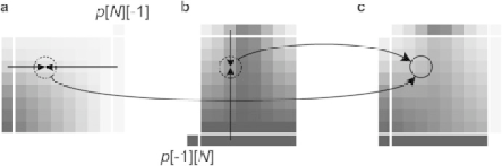
Fig. 4.7
Example of planar prediction: (
a
) illustrates calculation of the horizontal component,
(
b
) illustrates generation of the vertical component and (
c
) provides an example of a final planar
prediction created by averaging the horizontal and vertical components
In the case of directly vertical prediction, there may be discontinuities on the left
boundary of the block as the leftmost column of predicted samples replicate the
value of the leftmost reference sample above the block. Similar discontinuities can
occur on the top edge of the block when directly horizontal prediction is selected.
To reduce these discontinuities along the block boundaries, the boundary samples
inside the prediction block are replaced by the filtered values by considering the
slope at the edge of the block [
11
]. This boundary smoothing is applied only for the
abovementioned three intra modes (DC prediction, the exactly horizontal angular
mode 26 and the exactly vertical angular mode 10) and when the prediction block
size is smaller than 32
32. Different approaches for other modes and block sizes
were studied during the course of HEVC development, but this combination of
modes and block sizes was found to provide a desirable balance between coding
efficiency and complexity. As the prediction for chroma components tends to be
very smooth, the benefits of the boundary smoothing would be limited. Thus, in
order to avoid extra processing with marginal quality improvements the prediction
boundary smoothing is only applied to the luma component.
When the intra mode is equal to exactly vertical direction, the prediction samples
p
[0][
y
] with
y
D
0 :::
N
1 are modified by using the sample difference between
two reference samples
p
[
1][
1] and
p
[
1][
y
]as:
pŒ0Œy
D
pŒ0Œy
C
..p Œ
1Œy
pŒ
1Œ
1/ >> 1 / for y
D
0:::N
1
(4.21)
where clipping operation to restrict the computed value within the sample bit-
depth is omitted for simplicity. For the exactly horizontal direction, the boundary
smoothing is done in a similar way.
In the case of DC prediction, a three-tap [1 2 1]/4 smoothing filter is applied to
the first prediction sample p[0][0] by using the predicted DC value
dcVal
and two
neighboring reference samples,
p
[
1][0] and
p
[0][
1], as follows: