Java Reference
In-Depth Information
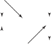
FIGURE 28-18
(a) A weighted graph and (b) the possible paths from vertex
A
to vertex
H
, with their weights
5
2
(a)
(b)
A
D
G
Path
Weight
4
1
2
A
A
A
A
A
B
B
D
E
E
E
E
G
F
H
F
H
H
H
H
9
9
8
10
10
1
6
B
E
H
3
1
3
3
4
1
C
F
I
28.22
Developing the algorithm.
The algorithm to find the shortest, or cheapest, path between two given
vertices in a weighted graph is based on a breadth-first traversal. It is similar to the algorithm we
developed for an unweighted graph. In that algorithm, we noted the number of edges in the path
that led to the vertex under consideration. Here, we compute the sum of the edge weights in the
path leading to a vertex. In addition, we must record the cheapest of the possible paths. Whereas
before we used a queue to order vertices, this algorithm uses a priority queue.
Note:
In a weighted graph, the shortest path between two given vertices has the smallest
edge-weight sum. The algorithm to find this path is based on a breadth-first traversal. Several
paths in a weighted graph might share the same minimum edge-weight sum. Our algorithm
will find only one of these paths.
Each entry in the priority queue is an object that contains a vertex, the cost of the path to that
vertex from the origin vertex, and the previous vertex on that path. The priority value is the cost of
the path, with the smallest value having the highest priority. Thus, the cheapest path is at the front
of the priority queue, and it is thus the first one removed. Note that several entries in the priority
queue might contain the same vertex but different costs.
At the conclusion of the algorithm, the vertices in the graph contain predecessors and costs that
enable us to construct the cheapest path, much as we constructed the path with the fewest edges
from the graph in Figure 28-16a.
28.23
Tracing the algorithm.
Figure 28-19 traces the traversal portion of the algorithm for the weighted
graph in Figure 28-18a when vertex
A
is the origin. Initially, an object containing
A
, zero, and
null
is placed in the priority queue. We begin a loop by removing the front entry from the priority queue.
We use the contents of this entry to change the state of the indicated vertex—
A
in this case—in the
graph. Thus, we store a path length of zero and a
null
predecessor into
A
. We also mark
A
as visited.
Ve r t e x
A
has three unvisited neighbors,
B
,
D
, and
E
. The costs of the paths from
A
to each of
these neighbors is 2, 5, and 4, respectively. These costs, along with
A
as the previous vertex, are
used to create objects that are placed into the priority queue. The priority queue orders these objects
so that the cheapest path is first.
We remove the front entry from the priority queue. The entry contains vertex
B
, so we visit
B
.
We also store within vertex
B
the path cost 2 and its predecessor
A
. Now
B
has vertex
E
as its sole
unvisited neighbor. The cost of the path
A
→
B
→
E
is the cost of the path
A
→
B
plus the weight of