Capillary Rise in a Taylor-Hauksbee Cell with a Tilted Edge - Selected Topics of Computational and Experimental Fluid Mechanics - page 513

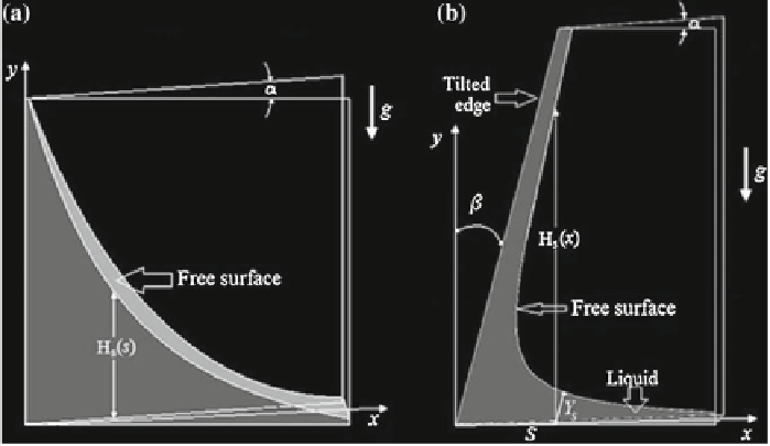
Fig. 1 a Scheme of the Taylor-Hauksbee cell. In this case the equilibrium profiles are given by

H s (

)

. b Taylor-Hauksbee cell with a tilted edge. In this case Y s is a distance to the equilibrium
profile along the line parallel to the tilted edge and that starts at x

x

= =

sandy 0; Thus the most

suitable coordinate system is given by ( s , Y s )

In order to compare the latter theoretical profile with experiments, we performed
a series of experiments with silicon oil of viscosity μ = 100 cP, surface tension

m 3 and an aperture angle of

˃ = ʱ =

0.0166 rad.
In experiments we used a digital Cannon Réflex T3i camera to take pictures and a
video recording of the capillary rise. In Fig. 2 we show a picture with the equilibrium
profile and also a comparison between the experimental data and the theoretical
profile given by Eq. ( 3 ). The fit is very good assuming that

0 . 0215N/m, density ˁ = 971 kg /

ʸ =

0 rad.

2.2 Cell with Tilted Edge

In this part we consider the cases of cells with tilted edges with respect to the ver-
tical, see Fig. 1 b. The usual Cartesian coordinates appears no suitable to depict the
equilibrium profiles because it is possible that for some values of x there are two
values of H ( x ) (the equilibrium profile). Thus, the concept of function can be lost.
Instead, we choose the rotated coordinate system x , y )

( to describe the equilib-

rium profile. We analyze the problem for the point ( s , Y s ) shown in Fig. 1 b. s is the

x y

distance from the lower apex to any point along x , whereas Y s is

the distance to the equilibrium profile along the line parallel to the tilted edge

( = 0 , = 0 )

y ) (

and that starts at the point x = and y = s cos ʲ s sin ʲ ; thus the equilibrium profile

is given by the injective function y ( x )

.