Environmental Engineering Reference
In-Depth Information
At the outlet, Neumann boundary conditions are used, that is,
∂
u
∂
v
x
=
x
=
0
,
at
x
=
X
L
,
0
≤
y
≤
H
.
(8)
∂
∂
At the side walls, we use no-slip conditions:
u
=
0
,
v
=
0
,
at
y
=
0
,
H
,
0
≤
x
≤
X
L
.
(9)
Here,
H
is the separation between lateral boundaries which determines the solid
blockage of the confined flow, characterized by the blockage parameter
H
.
In turn,
X
L
is the total length of the channel. The magnetic obstacles are located at
distances
X
u
from the entrance and
X
d
from the outlet. All the lengths are measured
in dimensionless units. The centers of the magnets are separated by a dimensionless
distance
D
ʲ
=
1
/
L
, where
d
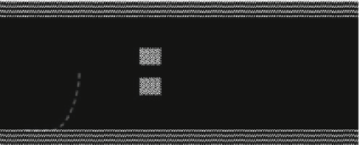
is the dimensional separation. Figure
2
shows a sketch
of the flow conditions considered for the numerical solution.
A finite volume method implemented with a SIMPLEC algorithm is used to solve
the governing equations (
3
)-(
6
) with boundary conditions (
7
)-(
9
). The diffusive and
convective terms are discretized using a central difference scheme. Accurate tem-
poral resolution is provided by choosing a small enough time step and employing a
second order scheme for the time integration. The numerical solution was obtained
in a rectangular domain with a length of
X
L
=
=
d
/
35 dimensionless units in the stream-
wise direction and
H
=
7 units in the cross-stream direction using an equidistant
orthogonal grid of 212
×
202 nodes. It was determined that an upstream distance
X
u
=
10 and a downstream distance
X
d
=
25 guarantee results that are nearly
independent of the location of the obstacles.
Electrode
u = v = 0
u
x
= 0
u = 1
v = 0
H
D
v
x
= 0
u = v = 0
y
Electrode
X
u
X
d
x
X
L
Fig. 2
Sketch of the geometry and boundary conditions considered for the analyzed flow


Search WWH ::

Custom Search