Geology Reference
In-Depth Information
20
18
ρ
= 0.9
0.8
Power law noise
10
1
16
0.7
0.6
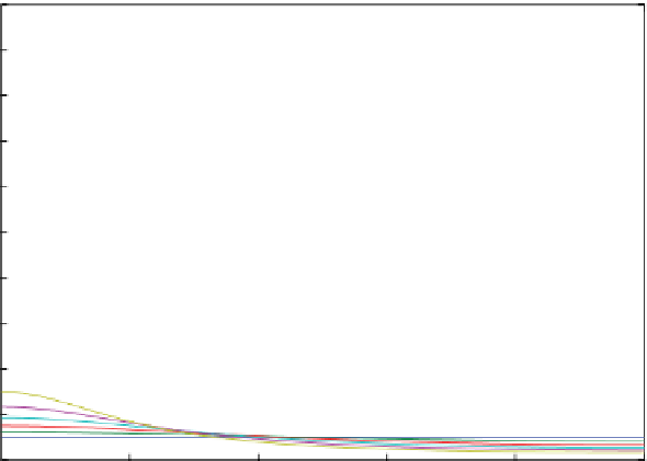
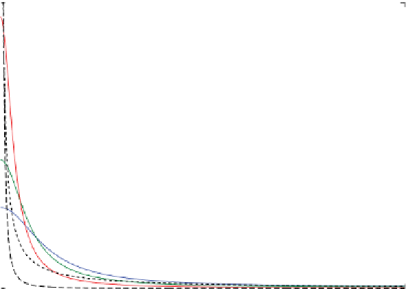
Figure 4.18
Spectral noise
models. The main plot
shows autoregressive
(Markovian) spectral noise
models (computed with
arnoisemodel.m
for different
values for ρ) and power law
noise models for 1/f and 1/f
2
(computed with
alphanoise.m
and rescaling the variance to 1,
i.e., that of the autoregressive
noise models), with 1:1 and 1:2
slopes in log
10
(power) vs.
log
10
(frequency), as depicted in
the inset.
0.5
0.4
0.3
0.2
0.1
14
ρ
= 0.9
10
0
0.0
1/f
12
Autoregressive noise
10
10
-1
Power law noise
1/f
2
8
1/f
10
-2
10
-3
6
0.8
1/f
2
10
-2
Frequency (1/n)
10
-1
4
0.7
Autoregressive noise
0.6
0.5
2
0.4
0.3
0.2
0.1
0.0
0
0
0.1
0.2 0.3
Frequency (1/n)
0.4
0.5
10
3
10
2
0.050
10
2
0.055
10
1
10
1
10
0
0
0.02
0.04 0.06
Frequency (1/n)
0.08
10
0
99%
10
-1
95%
90%
AR(1)
Estimated
ρ
= 0.9207
Actual
ρ
= 0.90
10
-2
0
0.1
0.2 0.3
Frequency (1/n)
0.4
0.5
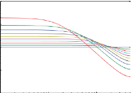
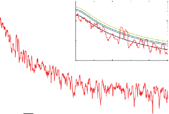
Figure 4.19
Hypothesis testing of the signal+red noise time series in Figure 4.17. The null model was calculated as
an AR(1) model using Husson's
reconf.m
. The 4π MTM adaptive weighted spectrum (red curve) was assigned a
constant 14 dof for all frequencies (dashed horizontal line in Figure 4.17), from which CLs were estimated at 85, 90,
95, and 99% levels. Instead of plotting each of these CLs with respect to the spectrum, the upper CL values were
applied instead to the AR(1) model, which on its own has 1000s of dof (thus has CLs that are not appreciably
different from the model estimate). This display is the convention that is used in the literature.