Geology Reference
In-Depth Information
21
4
3
2
1
0
0.2
0.15
0.1
0.05
0.0
0.15
0.1
0.05
0.0
0
-0.05
-0.1
-0.15
-0.2
0
-0.05
-0.1
-0.15
-0.2
0
2
π
3
π
20
40
60
80
100
20
40
60
80
100
n
n
(c)
(d)
0.2
0.15
0.1
0.05
0.0
0.2
0.15
0.1
0.05
0.0
6
5
1
4
2
3
0
-0.05
-0.1
-0.15
-0.2
0
-0.05
-0.1
-0.15
-0.2
0
4
π
5
π
20
40
60
80
100
20
40
60
80
100
n
n
(e)
60
1800
0.005
1600
5
π
18 dof's W=0.0024414
4
π
14 dof's W=0.0019531
3
π
10 dof's W=0.0014648
4
π
6 dof's W=0.0009765
FFT
2 dof's
Δ
f=0.0004883
50
1400
1200
40
1000
30
800
600
20
400
10
200
0
0
0
0.01
0.02
0.03
0.04
0.05
Frequency
0.06
0.07
0.08
0.09
0.1
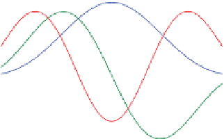
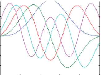
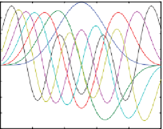
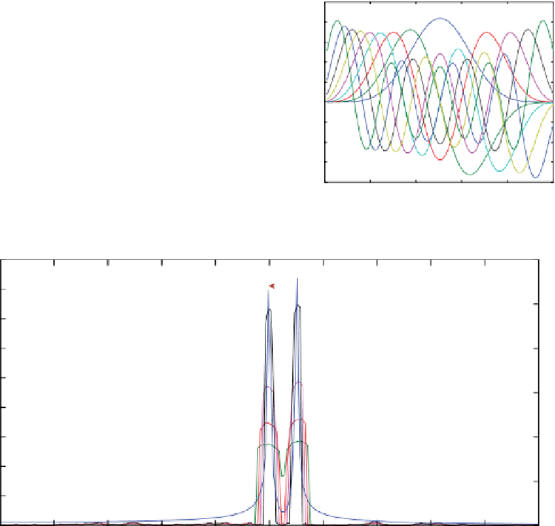
Figure 4.15
Examples of multitaper spectral estimators. Multitaper families (a-d) were calculated in MATLAB
using
dpss.m
, e.g., [E,V] = dpss(100,2) for 2π multitapers defined for a length of 100 points. The “E's” are the displayed
eigentapers, and the “V's” are the associated eigenvalues (not shown). Numbers indicate order. The tapers may be
rescaled to the length N and sample rate Δt of the time series that is to be tapered. The sum of the absolute values of
the tapers in a given family approximates a boxcar (Dirichlet) window. (e) [p,w] = pmtm(signal,2) for the 2π multitaper
power spectrum of the time series in Figure 4.10, and converting radial frequency w to linear frequency, f = w/(2πΔt),
is displayed for each of the multitaper estimators; the unsmoothed (Dirichlet) periodogram, designated as FFT, is
shown for comparison.