Geology Reference
In-Depth Information
(a)
+ 0.5
0
- 0.5
Dirichlet
Hann
+ 0.5
0
M=N
- 0.5
+ 0.5
0
- 0.5
M=0.5N
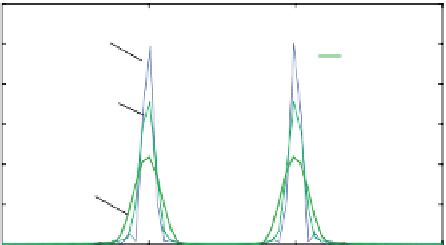
Figure 4.14
Autocorrelation
and the BT correlogram of
the test time series from
Figure 4.10. (a) Top:
Autocorrelation function of
the time series computed
from xcorr.m (xcorr(signal)
and normalized); middle:
autocorrelation function
multiplied by a Hann lag
window of length M = N;
bottom: autocorrelation
function multiplied by a
Hann lag window of
length M = 0.5 N. (b) BR
correlogram estimates of the
time series displayed in a;
effective dof are shown.
- 2000
-1000
0
Lag (n)
1000
2000
(b)
1200
Dirichlet
Hann
2 dofs
1000
800
5.33 dofs
(M =N)
600
400
10.67 dofs
(M = 0.5N)
200
0.045
0.05
0.055
Frequency (1/n)
0.06
spectral estimator”. D(n) is the data “lag” window applied analogously as in
the direct spectral estimator discussed above. The effective dof are larger for
smaller M, and defined in a straightforward way for windowed BT esti-
mates, per Fourier coefficient: N/M for the Dirichlet lag window, 3N/M for
the Bartlett lag window, and 8N/3N for the Hann lag window (e.g., Table 6.2
in Priestley (1981)).
BT correlogram estimation is illustrated in Figure 4.14 for the Dirichlet
and two Hann lag windows. The BT correlogram and direct spectral estimator
are not interchangeable: the autocorrelation function is naturally “tapered”
(owing to the limited length of the time series) and is twice as long
(N
ρ
= 2 × N - 1 = 4095), which results in a finer-scale FFT mesh. Thomson
(1977, 1990, 2009) warns that the BT correlogram can produce extremely
biased spectral estimates of some time series and advises against its use.
4.3.5.6 Thomson Multitapers
Over the past 50 years, dozens of single tapers have been designed to optimize
different aspects of spectrum estimation (e.g., Harris 1978). The objective of
all of these tapers is to control spectral leakage from the center lobe, increase