Information-Modeling Technology for the Environmental Monitoring - New Ecoinformatics Tools in Environmental Science: Applications and Decision-making - page 58

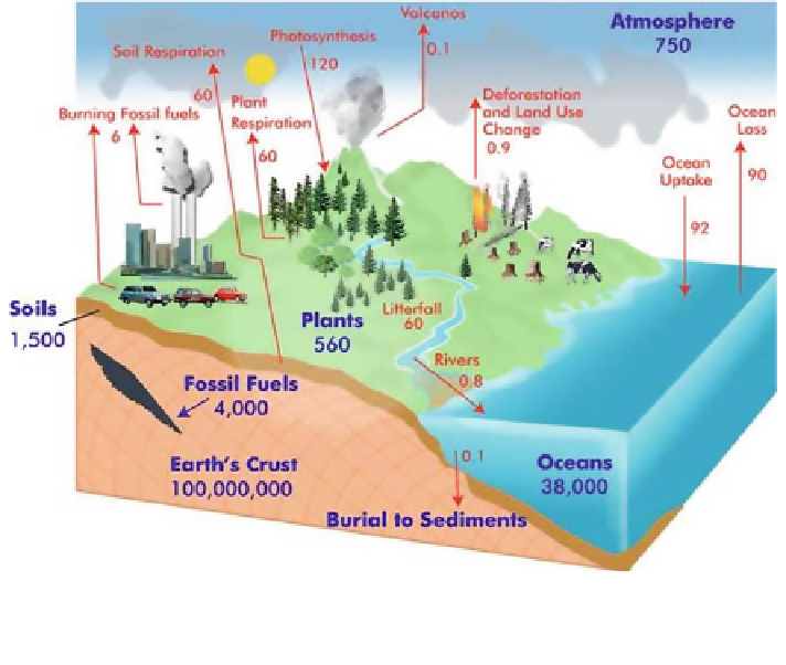
Fig. 1.23 A simplified diagram of the global carbon cycle. Pool sizes, shown in blue, are given in
petagrams (Pg) of carbon. Fluxes, shown in red, are in Pg per year ( http://www.globe.gov/projects/
carbon )

from 10 ppm at the South Pole to 15 10 ppm at the NH high-latitudes. This spatial

non-uniformity is explained by the presence in the Northern Hemisphere of large
seasonally photosynthesizing vegetation communities.
Diagram of the fast carbon cycle represented in Fig. 1.25 shows the movement
of carbon between land, atmosphere, and oceans in billions of tons of carbon per
year. Yellow numbers are natural

×

fluxes, red are human contributions in billions of
tons of carbon per year. White numbers indicate stored carbon. As it follows from
Figs. 1.23 , 1.24 and 1.25 latitudinal distribution of CO 2 in the atmosphere has non-
linear character. An increased CO 2 content in the NH atmosphere is closely con-
nected with the impact of human activity through direct CO 2 emissions and due to
the impact on vegetation cover. Almost 90 % of total carbon emissions due to
organic fuel burning fall on the zone 30 o N

fl

60 o N. It follows from the data in
Table 1.9 that the conceptual schemes of the global biogeochemical cycle of carbon
dioxide should also consider the spatial non-uniformity of atmospheric processes
(Kaminski et al. 2001).
An important constituent of most of the conceptual schemes of the global carbon
cycle is the structure of carbon

-

fluxes in the World Ocean. As follows from
Table 1.9 , there is a certain information possibility to select in the oceans several
layers by depths and to distinguish between the spatial non-uniformities in the
structure of the ocean surface. Most of the authors consider the vertical structure of

fl