Geoscience Reference
In-Depth Information
, and it thus follows that the average
number of observations in a sequential procedure equals to:
Accordingly, L(a
0
)=1
− α
and L(a
1
)=
ʲ
E
a
m
¼½
ð
1
aÞ
ln½
b=ð
1
aÞ þ a
ln½
ð
1
bÞ=a=
E
a0
n;
when a ¼ a
0
;
ð
3
:
9
Þ
E
a
m
¼½
b
ln½
b=ð
1
aÞ þ ð
1
bÞ
ln½
ð
1
bÞ=a=
E
a1
n;
when a ¼ a
1
2
> 0 we have:
For a=a* and when E
a*
ʾ
= 0 and E
a*
ʾ
2
E
a
m
ln
½
½
b=ð
1
aÞ
ln
ð
1
bÞ=a=
E
a
n
ð
3
:
10
Þ
According to Eqs. (
3.9
) and (
3.10
), the number of observations of a sequential
procedure is a random variable
m
, the average value of which (E
a
m
) can be smaller
or larger than n. It is necessary to have the distribution P(
m
= n)=P
a
(n) in order to
judge the possible values of
m
:
;
pÞ
1
=
2
exp
0
P
a
ðÞ
¼w
c
ðÞ
¼c
1
=
2
y
3
=
2
5cy
þ
y
1
E
a
m
ð
2
:
2
ð
3
:
11
Þ
where
2
0
y
nE
a
n
j
j
\
1;
c ¼ KE
a
n
j
j=
D
a
n
¼
ð
E
a
mÞ
=
D
a
m
[
0
;
3
D
a
m
¼ KD
a
n=ð
E
a
nÞ
;
E
a
m
¼ K
=
E
a
n;
K ¼ lnA for E
a
n
[
0 and K ¼ lnB for E
a
n
\
0
:
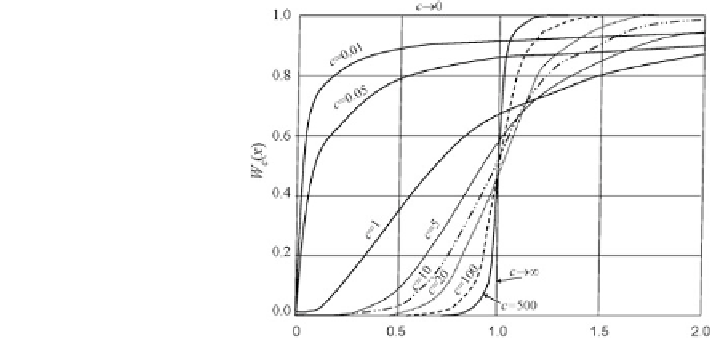
According to (
3.11
),
the Wald
'
s distribution function W
c
(y), has the form
(Figs.
3.3
and
3.4
):
Fig. 3.3 The Wald
'
s
distribution function
depending on the parameter c
Search WWH ::

Custom Search