Geography Reference
In-Depth Information
M
4
M
3
S
3
S
5
K
M
6
S
2
S
1
S
4
M
5
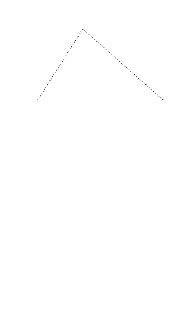
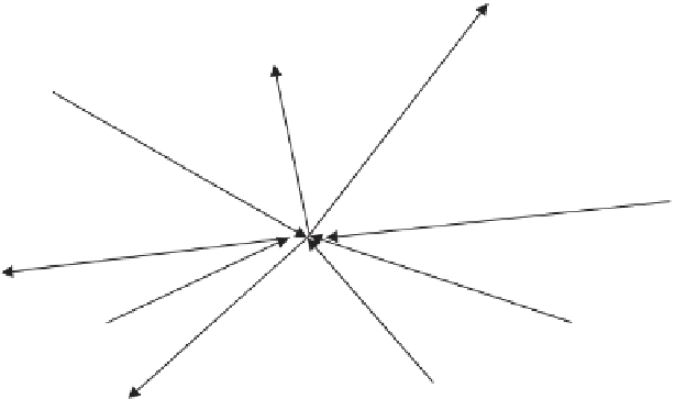
Figure 3.5
Polygonal location-production system
to hold for firms with more orthodox production functions which allow
for input substitution between the inputs sources from
S
1
,
S
2
,
S
3
and so on.
(Moses 1958; Khalili et al. 1974; Miller and Jensen 1978; Eswaran et al.
1981). Although the technical analysis of these models is beyond the scope
of this topic, it is interesting to highlight the main conclusions. In particu-
lar, firstly, where the prices of inputs and outputs
p
1
,
p
2
, and
p
3
are not only
exogenous but are also independent of the distance costs
t
1
,
t
2
,
t
3
, and so on,
the optimum location of the firm
K
* stays exactly the same even as the firm
expands its level of output, as long as the firm exhibits constant returns
to scale and also firm's expansion path is a straight line from the origin
(McCann 2001). This is the case where the firm's production function is
either linear, as in a Leontief function, or homogenous of degree one, as
in a Cobb-Douglas function. In other words, with these particular types of
production functions, once we calculate the firm's Weber optimum
K
*, this
will always remain the firm's optimum location whatever the firm's level of
output, as long as the location-specific labour prices and land prices do not
change. This is empirically a very useful insight, because the production
functions of many manufacturing firms in reality do have these particular
properties (Morroni 1992). In situations where as the firm expands its
output it tends to substitute in favour of one input and away from another
input, then the optimum location of the firm will tend to move towards the
input whose use is increasing faster as the output expands.