Geography Reference
In-Depth Information
M
3
d
3
K
d
1
d
2
S
1
S
2
Notes:
m
1
,
m
2
weight (tonnes) of material of input goods 1 and 2 consumed by the firm.
m
3
weight of output good 3 produced by the firm.
p
1
,
p
2
prices per ton of the input goods 1 and 2 at their points of production.
p
3
price per ton of the output good 3 at the market location.
S
1
,
S
2
production locations of input goods 1 and 2.
M
3
market location for the output good 3.
t
1
,
t
2
transport rates per ton-mile (or per ton-kilometre) for hauling input goods 1 and 2.
t
3
transport rates per ton-mile (or per ton-kilometre) for hauling output goods 3.
K
the location of the firm.
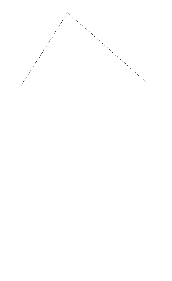
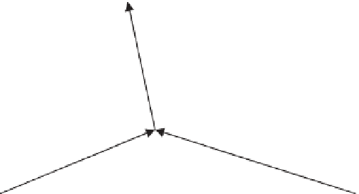
Figure 3.2
Weber location-production triangle
each input required in order to produce a single unit of the output. These
coefficients are assumed, for the purposes of this model, to be exogenously
given.
Our production function therefore takes the general form:
m
3
5
f
(
k
1
m
1
,
k
2
m
2
)
(3.1)
where
k
1
and
k
2
are fixed coefficients.
In order to develop the locational analysis we also assume that the
labour and capital input production factors are freely available every-
where at factor prices and qualities that do not change with location, and
that land is homogeneous. In other words, we assume for the moment that
the price and quality of labour is equal everywhere, as is the quality and
rental cost of land. This does not imply that the prices of labour and land
are equal to each other, rather that all locations exhibit the same attributes
in terms of their production factor availability. Geography and space are
therefore assumed to be homogeneous.
If the firm is able to choose to locate anywhere it wishes, in order to