Analyzing Stationary States of Gene Regulatory Network Using Petri Nets - Biological Petri Nets - page 154

Fig. 5. The ABC model. The expression of gene AP1 is responsible for the activity A , expression of genes AP3 , PI is responsible
for the activity B and expression of gene AG is responsible for the activity C .
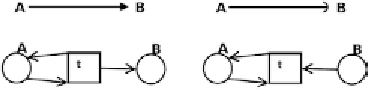
Fig. 6. Gene A activates or represses gene B , as shown by the arrow in the upper part of the left- and right-hand side diagram,
respectively. The bottom parts show how this is expressed in terms of Petri nets. Genes are denoted by places and the activation
relation is denoted by a proper transition.
The ABC model is broadly used to describe these different equilibria. According to the model there are
three types of activities (A, B and C) and their combination determines the type of the cell. Each activity
has genes associated with it. The activity is observable if in the equilibrium these genes are active.
Figure 5 illustrates the connection between activities, genes and flower parts (compare with Mendoza et
al. , 1999).
From gene regulatory network to a Petri net
Figure 4 shows the graphical representation of the gene regulatory network underlying flower morpho-
genesis of A. thaliana . The vertices represent genes and arrows represent the regulatory relations. In the
corresponding Petri net genes are represented by places and regulatory relations by transitions. Figure 6
present the rules for translating an ordinary regulatory network to a Petri net. After applying these rules
to the network from Fig. 4 we obtain a Petri net as the one shown in Fig. 7.
Stationary state analysis
This section presents an analysis of the stationary states of A. thaliana flower cells using Petri nets,
which have a uniform bound of 1 on all places (see section “ Petri nets with bounds ”). This models genes
being either active (1) or inactive (0).
First we discuss the genes involved in the morphogenesis and later we show two different approaches
to the analysis of the gene regulation network. Following [Mendoza and Alvarez-Buylla, 1998; Mendoza
et al. , 1999] we assume that the topology of the network is given. The first approach is to translate the
network to the Petri net and then find all the stationary states. In the second approach we restrict the set of
genes under question, translate to a smaller Petri net and find all the stationary states in that net. The first
approach requires no preprocessing, but heavy post-processing is needed. The second approach requires
one to restrict the set of analyzed genes, but yields results that require virtually no post-processing.
Moreover, the first approach can lead to loss of some significant information due to lack of information
on gene activity times. This is not the case in the second approach were the set of genes is by definition
restricted to non-temporary ones. In this refined approach we consider the network model “from the
developmental biology piont of view” and highlight only the subset of interactions occuring in given