Graphics Programs Reference
In-Depth Information
values of
x
at which we are sampling
u
, but since
u
(
x,t
) is pre-determined at
the endpoints, we can take
u
to be a 9-dimensional vector, and we just tack
on the values at the endpoints when we're done. Since we're replacing
∂
2
u
/∂
x
2
by its finite difference approximation and we've taken
x
=
1 for
simplicity, our equation becomes the vector-valued ODE
∂
u
∂
t
=
k
(
A
u
+
c
)
.
2
u
/∂
x
2
). The
Here the right-hand side represents our approximation to
k
(
∂
matrix
A
is
−
21
···
0
.
.
.
.
.
.
1
−
2
A
=
,
.
.
.
.
.
.
.
.
.
1
0
···
1
−
2
2
u
/∂
x
2
at (
n
,
t
) with
u
(
n
−
1
,
t
)
−
2
u
(
n
,
t
)
+
u
(
n
+
1
,
t
).
We represent this matrix in MATLAB's notation by
-2*eye(9) + [zeros(8,1),eye(8);zeros(1,9)] +...
[zeros(8,1),eye(8);zeros(1,9)]'
The vector
c
comes from the boundary conditions, and has 15 in its first
entry, 25 in its last entry, and 0s in between. We represent it in MATLAB's
notation as
[15;zeros(7,1);25]
The formula for
c
comes from the fact
that
u(1)
represents
u
(
−
4
,
t
), and
∂
since we are replacing
∂
2
u
/∂
x
2
at this point is approximated by
u
(
−
5
,
t
)
−
2
u
(
−
4
,
t
)
+
u
(
−
3
,
t
)
=
15
−
2
u(1)
+
u(2)
,
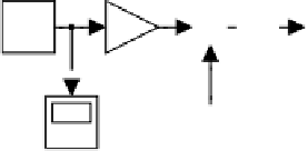
and similarly at the other endpoint. Here's a SIMULINK model representing
this equation:
1
s
Integrator
K*u
2
Gain
k
boundary
conditions
Scope
-C-
Note that one needs to specify the initial conditions for
u
as Block
Parameters for the Integrator block, and that in the Block Parameters dialog


Search WWH ::

Custom Search