Graphics Programs Reference
In-Depth Information
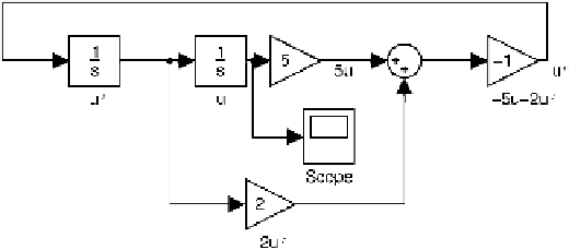
Figure8-4: A Finished SIMULINKModel.
the Integrator blocks and changing the line of the Block Parameters box that
reads “Initial condition”. For example, suppose we set the initial condition for
u
(in the first Integrator block) to 5 and the condition for
u
(in the second
Integrator block) to 1. In other words, we are solving the system
u
+
2
u
+
5
u
=
0
,
u
(0)
=
1
,
u
(0)
=
5
,
which happens to have the exact solution
u
(
t
)
=
3
e
−
t
sin(2
t
)
+
e
−
t
cos(2
t
)
.
Your first instinct might be to rely on the Derivative block, rather than the
Integrator block, in simulating differential equations. But this has two
drawbacks: It is harder to put in the initial conditions, and also numerical
differentiation is muchless stable than numerical integration.
Now go to the
Simulation
menu and hit
Start
. You should see in the Scope
window something like Figure 8-5. This of course is simply the graph of the
function 3
e
−
t
sin(2
t
)
+
e
−
t
cos(2
t
). (By the way, you might need to change the
scaleontheverticalaxisoftheScopewindow.Clickingonthe“binoculars”icon
does an “automatic” rescale, and right-clicking on the vertical axis opens an
Axes Properties...
menu that enables you to manually select the minimum
and maximum values of the dependent variable.) It is easy to go back and
change some of the parameters and rerun the simulation again.
Finally, suppose one now wants to study the
inhomogeneous
equation for
“forced oscillations,”
u
+
2
u
+
5
u
=
g
(
t
), where
g
is a specified “forcing” term.
Search WWH ::

Custom Search