Travel Reference
In-Depth Information
B
130
128
120
110
AB
best fit
=
line of
100
(Yr. 3)
(Yr. 2)
90
80
A
(Yr. 1)
7000
7500
8000
8300 8500
projected
income
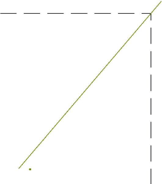
Figure 13.2
Relationship between
income and travel demand.
Per Capita Income of Tourists ($)
and prices) and obtain a mathematical relationship between them. To estimate future demand,
projected income and price levels for the relevant year can simply be substituted into the
mathematical formula. The resulting estimate of demand will be more reliable than will one obtained
by the simple regression method, because the former incorporates the combined effect of income and
price on demand.
Indeed, the analysis is not restricted to these two variables alone. Conceptually, any number of
variables can be used to explain and predict demand levels. But there are some practical limitations. As
the number of
variables increases, the calculations become increasingly complex. In
addition, the costs involved in collecting the additional data and solving the mathematics of the
technique are considerable. In some instances, the incremental reliability of the estimates may not
justify these expenses, because estimates are after all only estimates and are not certain to
materialize
''
explanatory
''
no matter how comprehensively they may be calculated.
In addition to the expense involved, another drawback of multiple regression is that the
relationships cannot be depicted graphically, as the results of the two earlier methods can be.
The reason is, of course, that we get into multidimensional planes. Up to three dimensions can
be depicted visually, but beyond that it becomes impossible.
—
Computer Simulations and Models
Another projection method is to build a computer model that will simulate tourist demand. Typically,
the demand for tourism to a particular area is a function of factors such as levels of income of tourists,
the cost of travel from the tourists
'
homes to the destination, price levels, competition, currency


Search WWH ::

Custom Search