Geology Reference
In-Depth Information
local maximum correlation. This is shown by the box with
the dark boundary in Figure 10.45b. The displacement of
the subarea can then be represented by the vector that con-
nects the centers of the matched windows in both images as
shown in the figure. Matching windows with higher values
of
R
are better than those with lower values. The displace-
ment vectors can be established at any number of points
in the first image where matching features are available.
Alternatively, the common practice is to use a uniform grid
overlaid on the first images and find their matches in the
second image. The displacement vectors will be established
for the points that have unique structure to allow finding a
match. For the rest of the grid points the vectors can then
be established by interpolation or extrapolation. This is
shown in Figure 10.45c. The average velocity
V
of the grid
point over the intervening time interval between the two
images can be obtained directly from the displacement of
the point using the simple equation
[
Heacock et al
., 1993]. The software was applied to a
variety of satellite imagery including AVHRR, ERS,
SSM/I, and Radarsat.
Agnew et al
. [1997] applied it to
track ice motion in the entire Arctic basin using the SSM/I
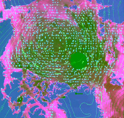
85 GHz channel data. Figure 10.46 shows vectors of ice
displacement estimated from the data for the 4 day period
(20‐24 December 1993). The vectors are presented on
an Eulerian grid (the difference between Eularian and
Lagrangian grids is explained later). The strong anticy-
clonic circulation of the Beaufort Sea Gyre is apparent.
Not many points are shown in the Fram Strait (east of
Greenland), but the few points shown do not replicate the
high velocity shown by the drifting buoy motions. Ice
velocity in this area is typically large. The background
image in Figure 10.46 is the 85 GHz SSM/I image for 20
December 1993. The superimposed sea level pressure
pattern demonstrates that ice motions are mainly forced by
atmospheric wind.
Agnew et al
. [1999] used the Ice Tracker
again to study the formation of coastal leads in the
Canadian Archipelago off the Prince Patrick Island in the
western Arctic where the mean position of anticyclonic
flow over the Beaufort Sea begins to set up strong shearing
forces into the ice pack. The study used the same observa-
tions from the SSM/I 85.5 GHz channel. It confirmed that
xt xt
t
i
1
i
V
(10.109)
t
i
1
i
where
x
denotes the position of the point in the initial
image (at time
i
) and the next image (at time
i
+ 1).
The MCC method may involve other steps. A nested
correlation approach is used to reduce the computa-
tional burden. In this approach the correlation is per-
formed between the given pair of images but at a recursive
degrading resolution using average filtering with (
m
×
m
)
pixel. The size of the filter varies using four stages of
resolution defined by
m
= 81, 27, 9, and 3. The algorithm
can also be applied to regularly spaced grid points. A
strategy that avoids searching over the entire scene to find
a maximum correlation starts by applying the correlation
on seeds of control points that can be identified in the
pair of the coarsest resolution images. These can be the
brightest areas in each image. The first set of tie points
can then be identified. In the rest of the algorithm the tie
points are established at as many grid points as possible
by interpolating between existing tie points. The process
continues as the algorithm proceeds through the hierar-
chical stages from one resolution image pair to the next.
Fily and Rothrock
[1987] applied the algorithm to two
pairs of Seasat SAR images acquired in October 1978.
They confirmed that the accuracy of the motion field
improved as the stages of calculations advance. They also
suggested that the algorithm would perform poorly on
highly fragmented ice floes. A more serious limitation of
the MCC method is its inability to capture the rotational
component of sea ice motion.
The MCC technique was implemented in the first ver-
sion of automated software called Ice Tracker, which was
used by the Canadian Ice Service to track ice motion
25 km/day
Greenland
Figure 10.46
Four day (20-24 December 1993) sea ice motion
vectors over the Arctic basin obtained from daily averaged
85.5 GHz SSM/I data using the Canadian Ice Tracker software.
Small yellow circles mark the beginning of the ice motion
and the length of line represents the speed. Vectors in red
are drifting buoy motions. The loci of sea level pressure con-
tours are superimposed [
Agnew et al
., 1997]. (For color detail,
please see color plate section).