Geology Reference
In-Depth Information
300
280
260
240
220
200
180
160
140
120
100
Tb-19V
Tb-19H
1 cm snow + 1.6 cm ice
3 mm slush + 1 cm snow-ice + 4 cm saline ice
3 mm fresh-water ice
+3 cm saline ice slush
-8.1°C
Tb-37V
Tb37-H
-3.4°C
-5.2°C
Tb-85V
Tb-85H
34 ppt
14 ppt
-6.3°C
3 cm slush. 98% ice
-0.5°C
+ 8.6°C
8 cm snow on OW
3 cm snow
Freezing rain
3 ppt
Rain over 2 cm candied ice
1 cm snow
110
100
90
80
70
60
50
40
30
20
10
0
NT2
ASI
BSA
NT
110
100
90
80
70
60
50
40
30
20
10
0
ECICE-19GHz
ECICE-37GHz
ECICE-85GHz
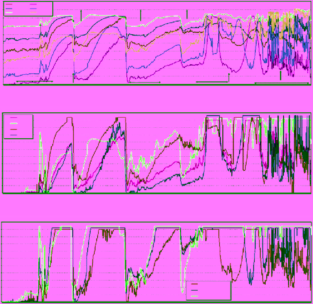
Figure 10.24
Evolution of measured brightness temperature from laboratory‐grown simulated sea ice (top) and
the derived ice concentration using the indicated four algorithms (middle) and the ECICE algorithm with three
sets of input observations (bottom). The input to ECICE is explained in the text. The horizontal axis shows the
day of the year, hour, and minute in the format (ddd:hh.mm). Upward arrows indicate the time associated with
the information next to the arrow [
Shokr and Kaleschke
, 2012]. (For color detail, please see color plate section).
Greenland, and Barents Seas). It should be noted that
passive microwave observations are more affected by
atmospheric influences in areas of low ice concentration.
Moreover, the differences in spatial resolutions of the
sensors used by different algorithms will certainly con-
tribute to differences in the results. In late summer
(September) the study found that the deviation between
algorithms was large (reaching 12%) in the Canadian
Archipelago region. This time of year is characterized by
the presence of melt pond on ice surface and MY ice drift
from the central Arctic through certain passages to south-
ern areas. The study concluded that results from the algo-
rithms that use the same category of frequency channels
(low or high) are correlated more. Based on the passive