Geology Reference
In-Depth Information
single circularly-polarization signal (mostly right-circular
R) and receives two linear orthogonal signals (e.g., RH
and RV). Parameters derived from the CP backscatter
(combining intensity and phase measurements) should be
assessed for their potential use in sea ice classification.
This potential has been predicted in a preliminary review
on the future applications of the data [
Charbonneau et al
.,
2010]. The first trial to explore the best CP parameters
for ice classification has been presented by
Dabboor
and Gledsetzer
[2013]. The authors applied a maximum-
likelihood classification approach using different combi-
nations of CP parameters and determined the best
combination based on the classification error. A few CP
parameters outperformed the linear polarization param-
eters. More studies on CP data are expected to emerge in
preparation for their availability from future SAR sys-
tems such as the one scheduled for launch in 2018
onboard the Canadian Radarsat Constellation Mission.
This system will acquire CP data in the ScanSAR mode.
The potential of using multifrequency SAR data for
ice type classification has been explored in
Brath et al
.
[(2013)] using the Wishart metric [equation (10.10)].
They used multifrequency co‐polarization (HH and VV)
data acquired by a helicopter‐borne scatterometer during
the German R/V Polarstern cruise ARKXXII/2 into the
eastern Arctic Ocean in October 2007 (early freezing
period). Classification was performed to identify four ice
types: new ice < 10 cm thick (N), gray Ice between 10 and
15 cm thick (GI), old ice (OI), and OW (no FY ice was
found during the expedition). For training the supervised
Wishart classifier, covariance matrices composed of HH
and VV backscattering were obtained from training sets
of the ice types. The authors presented an extensive set
of histograms of
0
for seven intervals of inci-
dence angles for each ice class at four scatterometer
microwave frequencies: S‐, C‐, X‐, and Ku‐bands (see
Table 7.1 for frequencies and wavelengths). The unique
contribution of the study was to determine the relative
performance of the single frequency and combination of
frequencies for ice classification. All possible combina-
tions of the aforementioned frequencies were tested.
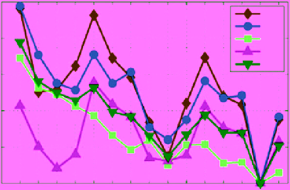
Figure 10.9 shows the accuracy of classification of each
ice type and the overall classification accuracy from 15
single and combined frequency channels. These accura-
cies were calculated with respect to the accuracy from
using the combination CXKu (a symbol for the combined
C‐, X‐, and Ku‐bands), which was assumed to be the
“best accuracy” based on visual observations and video
images of the scene. In other words, the absolute accu-
racy from each frequency setting could not be determined
because of the lack of independent quantitative truth
data (quantitative ice‐type estimate using an IR sensor
onboard the same helicopter failed due to warm ice
surface). However, a few important observations can
be derived from Figure 10.9. Using a single frequency,
the classification accuracy improves as the frequency
increases (except for the fact that the Ku‐band degrades
the classification with respect to the X‐band). The same
0
and
hh
vv
50
N
Gl
Ol
Ow
all
40
30
20
10
0
Figure 10.9
Relative classification accuracy of three ice types plus OW using Wishart classifier from multi-
polarization helicopter‐borne scatterometer data (S‐, C‐, X‐, and Ku‐band). The combination CXKu is used as the
reference from which relative classification accuracy (difference %) is estimated. The combinations of frequencies
shown in the labels of the horizontal axis are supposed to be aligned with the vertical dotted line [
Brath et al
.,
2013, Figure 14, with permission from IEEE].