Geology Reference
In-Depth Information
90°W
90°E
H
Alaska
1 May 1985
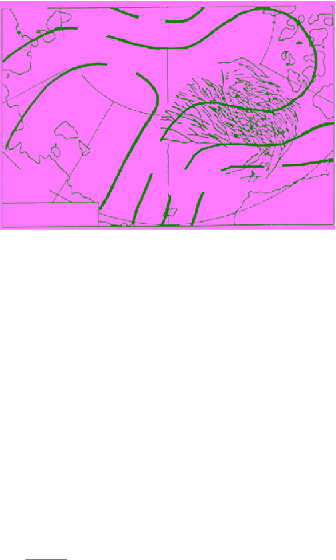
Figure 9.9
Mean sea level pressure (mbars) pattern in the Beaufort Sea on 1 May 1985 and the lead distribution on
the following day using the VIS and TIR channels of the DMSP satellite (thin lines and curves). Note the tendency
of lead orientation to be arranged roughly parallel to the geostrophic wind direction, which is approximately paral-
lel to the isobars [adapted from
Barry et al.,
1989].
brightness temperature in winter and albedo in summer.
For each cell of 200 km
2
they calculated the surface tem-
perature
T
sfc
using a split‐window technique (section 7.5).
In a heterogeneous pixel, a potential for open water based
on a temperature ratio denoted
δ
BT
can be calculated
using typical values of temperature of thick ice
T
ice
and
open water
T
ow
selected threshold. Based on
δ
BT
or
δ
A
equal to 0.1,
Lindsay and Rothrock
[1995] found that the average lead
width in the central Arctic reaches a minimum of 2.3 km
in January and February and a maximum of 6 km in
September. They also confirmed a previous finding by
Wadhams
[1988] that the distribution of lead width fol-
lows a power law (the power law distribution exhibits a
negative exponential shape when plotted on a linear axis
system and a linear shape when plotted on log‐log axes)
TT
TT
sfc
ice
TT
(9.9)
BT
sfc
ice
ow
ice
Naw
b
(9.12)
()
w
and
where
N
(
w
) is the number of leads of width
w
per kilom-
eter of track and
a
and
b
are coefficients that can be
determined from empirical data (the best fit of frequency
of occurrence of lead width from a set of lead width
measurements).
Wadhams
[1988] used submarine sonar
data to calculate a power law exponent,
b
= 2, in Fram
Strait and
b
= 2.29 in Davis Strait.
Using a threshold on satellite radiometric measurements
to identify leads produces better results when the leads are
open. In winter, leads in polar areas almost certainly con-
tain thin ice types due to rapid refreezing. This renders their
detection using a single threshold inadequate. Moreover,
mixed pixels from medium‐resolution imagery data (e.g.,
MODIS and NPOESS sensors), which are commonly used
for lead detection, cannot be interpreted correctly using the
binary product of the threshold technique. To account for
these considerations and to develop an algorithm capable
of detecting narrow leads,
Onana et al.
[2013] developed an
0
TT
(9.10)
BT
sfc
ice
Similarly, the potential for open water, based on albedo,
denoted
δ
A
, is given by
ice
sfc
(9.11)
A
ice
ow
where
α
sfc
is the estimated surface albedo from AVHRR,
α
ice
and
α
ow
are the typical albedo of ice and open water;
respectively.
Lindsay and Rothrock
[1995] used
δ
A
for the
summer months June, July, and August. When a thresh-
old of
δ
BT
or
δ
A
is chosen, binary images of lead‐like
structures can be generated. Statistics of leads (e.g.,
length, width, orientation, and spatial frequency) can
then be determined, but they will be sensitive to the