Geology Reference
In-Depth Information
51°N latitude on 16, February 1992. Figure 8.18 shows
the variation of PR
37
and GR
19
V
37
V
across the ice edge in
the Labrador Sea as identified by ice analysts in the
Canadian Ice Service. The sharp drop, particularly in the
polarization ratio, from OW to ice is clearly observed. This
drop is not as sharp in the case of higher frequency chan-
nels (e.g., PR
85
) as shown in
Shokr et al
. [2009]. Polarization
ratio is usually used as a criterion to discriminate between
sea ice and OW while gradient ratio is used to filter out
OW pixels [
Markus and Cavalieri
, 2000;
Shokr et al
., 2008].
Cavalieri
[1994] used PR
19
and GR
19
V
37
V
in an algorithm
to estimate ice concentration taking into account the
presence of thin ice. These parameters became widely
used in subsequent algorithms. The author plotted the tie
points of the two parameters for three surfaces: OW, FYI,
and MYI using data obtained from SSM/I channels over
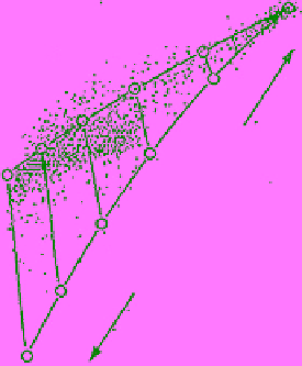
the Arctic in the winter of 1988. The plots (Figure 8.19)
are known as NASA's tie point triangles. This is a curvi-
linear triangle connecting the three tie points at its verti-
ces. Each side of the triangle is generated from calculations
of
T
b
using the following equation:
case of 60% FY ice, 40% OW, and 0% MY ice. Any point
inside the triangle will have a combination of the three
surfaces. On the other hand, any point falling outside
the triangle will produce an unrealistic combination of
ice type concentrations (i.e., >100% or <0%) if a set of
equations similar to equation (8.12), pertaining to differ-
ent observation, is to be solved. This issue will be discussed
further in section 10.2.2. A main point about the plots in
Figure 8.19 is the spread of the observation points in the
given parameter space. In the central Arctic, where there
is virtually no OW in winter, the scattered data points
are centered along the 100% ice concentration line, shared
between FY and MY ice. An algorithm based on the
shown triangle should estimate the ice concentration cor-
rectly in that region. On the contrary, the clustering of
the data from the Bering Sea is rather cumbersome. Here,
the ice cover features mostly thin types (<30 cm thick).
The data points reveal wide scattering with a tendency to
form a cluster with GR
19
V
37
V
values close to zero. More
sporadic distribution is observed along the line (OW‐
FY). According to
Cavalieri
[1994], it is not clear whether
this distribution is due to the presence of thin ice types or
to an actual mixture of thicker ice types (FY ice) with
open water. It could also be due to water vapor contents
in the atmosphere, generated by the large area of OW in
that region. As for the data from the entire Arctic, their
cluster around the OW tie point represents not only
OW but also weather‐related effects. It is possible that
the scattering of the points along the FY‐OW line could
represent measurements from young ice types. Brightness
TCTCTCT
b
(8.12)
OW
b
,
OW
FY
b
,
FY
MY
b
,
MY
The two sides of OW‐MY and OW‐FY are shown in
the figure with points marking ice concentration at a con-
stant interval of 20%. For example, the point marked
60% on the line OW‐MY represents the case of 40% OW,
60% MY ice, and 0% FY ice. The corresponding point on
the opposite side (i.e., the OW‐FY line) represents the
(a)
(b)
(c)
0.10
OW
OW
OW
0%
0%
0%
0.05
20%
20%
20%
FY
0.0
40%
FY
40%
40%
FY
60%
60%
60%
-.05
80%
80%
80%
Bering
Sea
Entire
Arctic
Central
Arctic
MY
MY
MY
100%
100%
100%
-0.1
0
0.1
0.2
0.3 0
0.1
0.2
0.3 0
0.1
0.2
0.3
PR
19
PR
19
PR
19
Figure 8.19
Polarization versus gradient ratios derived from SSM/I observations over (a) the entire Arctic,
(b) Central Arctic, and (c) Bering Sea, all obtained from SSM/I observations on 4 April, 1988 [adapted from
Cavalieri
, 1994, Figure 2, with permission from AGU].