Geology Reference
In-Depth Information
(a)
20 mm
(b)
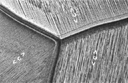
Figure 4.17
Optical micrograph of a replica of pure S2 ice
showing a triple point and different orientations of the
c
axis
(<
c
>) indicated by the long directions of the elongated etch pits
corresponding to basal dislocations intersecting the surface;
note the characteristics of the nearly symmetric grain boundary
in the right half of the micrograph and the two asymmetric grain
boundaries in the left (N. K. Sinha, unpublished).
20 mm
Figure 4.16
Photographs of double‐microtomed (DMT) thin
sections of pure S2 ice under cross‐polarized light: (a) horizon-
tal and (b) vertical; The scale bar in the images is 20 mm [
Sinha
et al.,
1996].
along the grain boundaries as well as on the surfaces of
the grains due to localized melting and refreezing.
The distributions of dark and bright objects in hori-
zontal sections of transversely isotropic S2 ice under
cross‐polarized light, such as Figure 4.16a, should change
evenly if the thin section is rotated while keeping the
cross polarizers in a fixed position. The grains with their
c
axis parallel to the pass direction of either the polarizer
or the analyzer (see section 6.1 for details on polari-
scopes) will appear as dark. Grains with their
c
axis ori-
ented at 45° to the pass direction of either of the two
polarizing sheets appear as bright. Thus, the randomness
of the
c
‐axis orientation can be judged very easily by
rotating horizontal thin sections under cross polarizers.
The
c
axis of the individual grains can be determined
exactly by installing the thin section on a universal stage
in between the polarizer and the analyzer, and perform-
ing the analysis for textural analysis and making fabric
diagrams [
Langway,
1958]. The procedures are rather
laborious and time consuming. However, a simple and
unambiguous method for quickly ascertaining (and
record keeping purposes) the randomness of
c
‐axis ori-
entations in S2 ice for selection of specimens for creep
and strength tests was developed by
Sinha
[1978b]. The
method can be applied, if deemed necessary, to each
test specimens in the form of large rectangular prisms
Figure 4.18
Horizontal, 100 mm diameter, thin section of first‐
year S2 sea ice from the Labrador Sea, photographed between
crossed polarizers; note the random orientation of the grains
and the corresponding orientation of the intragranular brine
inclusions (photo by M. Shokr, unpublished).
(preferred for columnar ice) with dimensions of 100 mm
× 250 mm × 50 mm before testing. It's based on chemical
etching and replicating the surface, as described in sec-
tion 6.4.4. An example is shown here in Figure 4.17.
The S2 type of transversely isotropic ice can also grow
in saline waters if there are no turbulences or tidal cur-
rents in the water. It has been seen to grow in protected
bays of saline or brackish water. Figure 4.18 shows S2‐
type sea ice formed in calm water in Labrador Sea near
Cartwright. The ice was sampled in March 1996 when