Global Positioning System Reference
In-Depth Information
1
2
3
4
5
6
7
8
9
10
11
12
13
14
15
16
17
18
19
20
21
22
23
24
25
26
27
28
29
30
31
32
33
34
35
36
37
38
39
40
41
42
43
44
45
[97
Lin
—
0
——
No
PgE
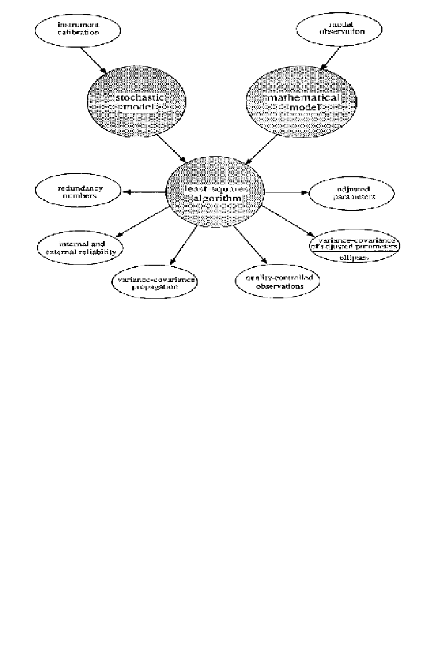
Figure 4.2
Elements of least-squares adjustment.
[97
Typically we do not use a subscript to identify
P
as the weight matrix of the observa-
tions. The symbol
0
denotes the a priori variance of unit weight. It relates the weight
matrix and the inverted covariance matrix. An important capability of least-squares
adjustment is the estimation of
σ
2
0
and it is the a posteriori variance of unit weight. If the a priori and a posteriori vari-
ances of unit weight are statistically equal, the adjustment is said to be correct. More
on this fundamental statistical test and its implications will follow in later sections.
In general, the a priori variance of unit weight
0
from observations. We denote that estimate by
σ
σ
0
is set to 1; i.e., the weight matrix is
equated with the inverse of the variance-covariance matrix of the observations. The
term
variance of unit weight
is derived from the fact that if the variance of an obser-
vation equals
σ
0
, then the weight for this observation equals unity. The special cases
that
P
equals the identify matrix,
P
σ
I
, frequently allow a simple and geometrically
intuitive interpretation of the minimization.
The mathematical model expresses a simplification of existing physical reality.
It attempts to express mathematically the relations between observations and pa-
rameters (unknowns) such as coordinates, heights, and refraction coefficients. Least-
squares adjustment is a very general tool that can be used whenever a relationship
between observations and parameters has been established. Even though the math-
ematical model is well known for many routine applications, there are always new
=