Global Positioning System Reference
In-Depth Information
1
2
3
4
5
6
7
8
9
10
11
12
13
14
15
16
17
18
19
20
21
22
23
24
25
26
27
28
29
30
31
32
33
34
35
36
37
38
39
40
41
42
43
44
45
Figure 9.14
Accuracy of the
∆
t
functions.
s
can be verified similarly. First, we map
the center of the geodesic circle and the polygon vertices using the direct mapping
equations. Next, we compute the map distances
d
i
between the mapped center and
mapped polygon points, and form the difference
The accuracy of the expressions for
∆
[33
s
i
−
d
i
. The subscript
dm
indicates that these values were obtained by using the direct mapping equations.
Next, the values
∆
s
i,dm
=
Lin
—
1.2
——
No
PgE
s
i
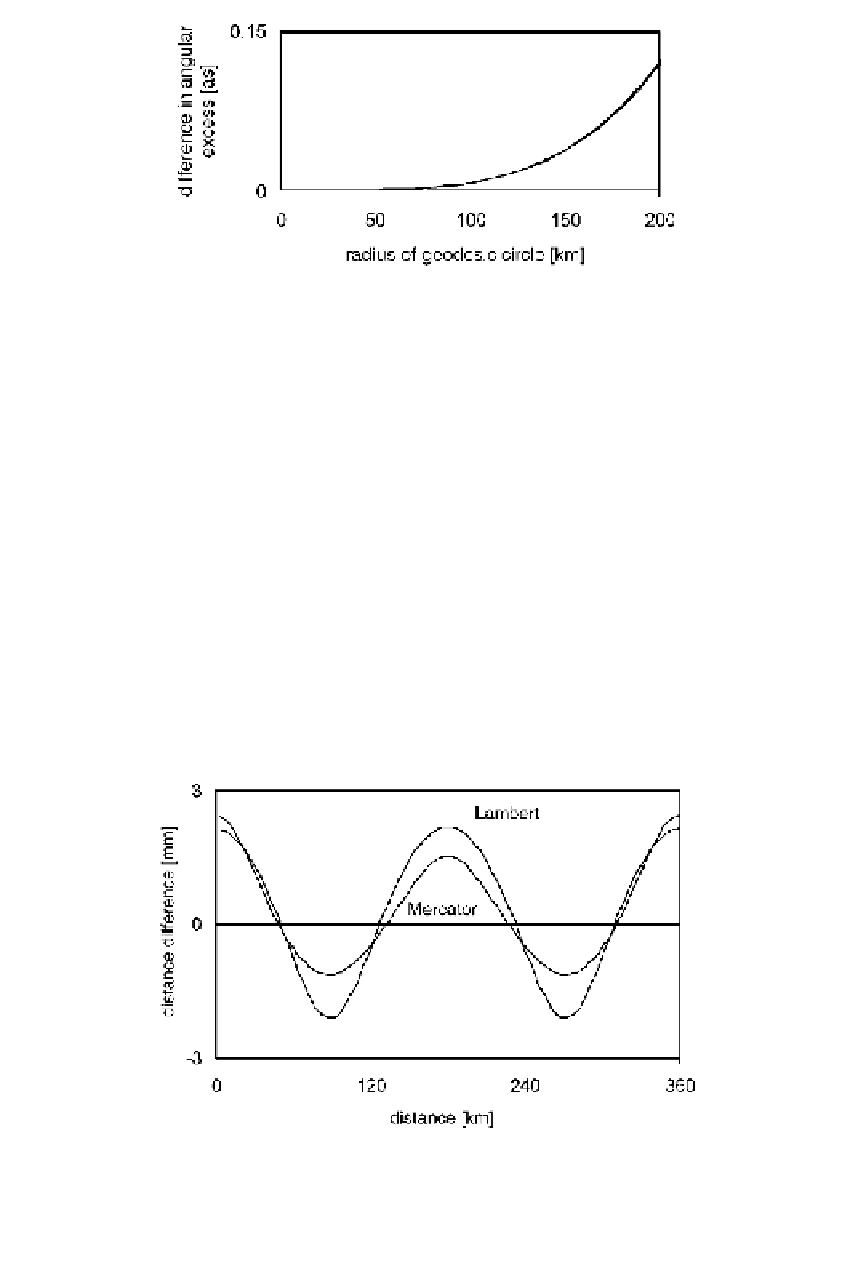
are computed from the explicit expressions in Table 9.5. Figure
9.15 shows the differences
∆
s
i,dm
for both TM and LC. The same conformal
mapping specifications have been used as given above, and, again, the radius of the
geodesic circle covers up to 2°. The figure demonstrates millimeter-level agreement
in the range of the test area.
Expressions for
∆
s
i
− ∆
∆
t
and
∆
s
that are even more accurate are available in the litera-
ture.
[33
9.2.6 Similarity Revisited
In
Appendix C, the conformal property is identified as similarity between infinites-
im
ally small figures. It is, of course, difficult to interpret such a statement because
Figure 9.15
Accuracy of the
∆
s
functions.