Global Positioning System Reference
In-Depth Information
1
2
3
4
5
6
7
8
9
10
11
12
13
14
15
16
17
18
19
20
21
22
23
24
25
26
27
28
29
30
31
32
33
34
35
36
37
38
39
40
41
42
43
44
45
[31
Lin
—
-1.
——
Nor
PgE
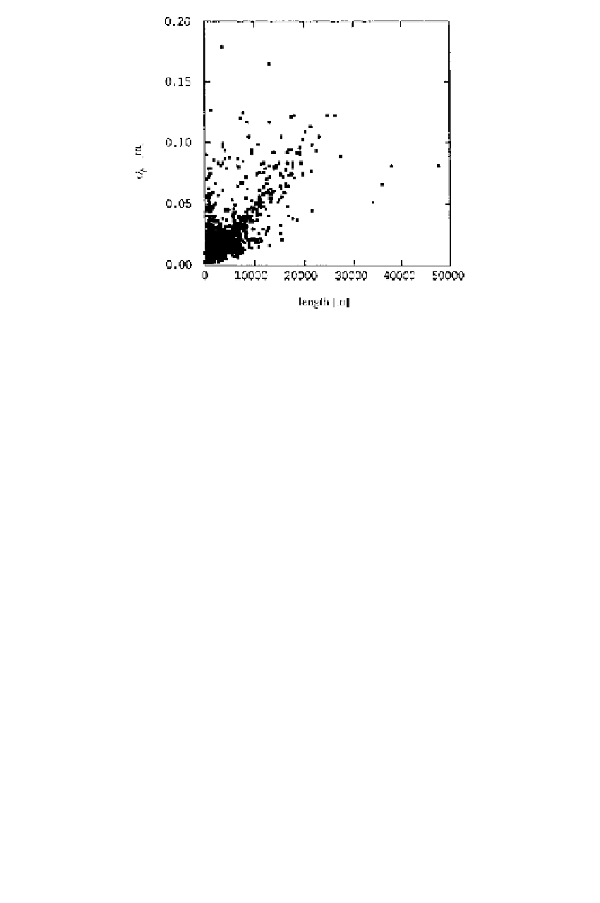
Figure 8.7
A priori precision of length of baseline.
(Permission by ASCE.)
m
atrix. Figure 8.7 displays
σ
k
as a function of the length of the vectors. For longer
lin
es, there appears to be a weak length dependency of about 1:200,000. Several
of
the shorter baselines show larger-than-expected values. While is not necessarily
de
trimental to include vectors with large variances in an adjustment, they are unlikely
to
contribute to the strength of the network solution. Analyzing the averages of
σ
[31
k
fo
r all vectors of a particular station is useful in discovering stations that might be
co
nnected exclusively to low-precision vector observations.
Va
riance Factor
Figures 8.8 and 8.9 show the square root of the estimated variance
fa
ctor
f
k
for each vector
k
. The factor is computed from
v
k
v
k
R
k
f
k
=
(8.29)
with
=¯
r
k
1
+¯
r
k
2
+¯
≤
≤
R
k
r
k
3
0
R
k
3
(8.30)
where
v
k
denote the decorrelated residuals and
r
k
3
are the redundancy
numbers of the decorrelated vector components. See Equation (4.375) regarding
the decorrelation of vector observations. The estimates of
f
k
are shown in Figures
8.8 and 8.9 as a function of the baseline length and the a priori statistics
r
k
1
,
¯
¯
r
k
2
, and
¯
σ
k
. The
scale factor
f
k
in Figure 8.10 is computed following the procedure of automatic
deweighting observations discussed in Section 4.11.3 (i.e., if the ratio of residual and
standard deviation is beyond a threshold value, the scaling factor is computed from