Global Positioning System Reference
In-Depth Information
1
2
3
4
5
6
7
8
9
10
11
12
13
14
15
16
17
18
19
20
21
22
23
24
25
26
27
28
29
30
31
32
33
34
35
36
37
38
39
40
41
42
43
44
45
constants and not included in
x
a
. The mathematical model
a
=
f
(
x
a
)
is very simple
in this case. The
n
components
f
will contain the functions:
x
i
−
x
j
2
+
y
i
−
y
j
2
d
ij
=
(4.382)
tan
−
1
x
k
−
x
i
tan
−
1
x
j
−
x
i
a
jik
=
y
i
−
(4.383)
y
k
−
y
j
−
y
i
In these expressions the subscripts
i
,
j
, and
k
identify the network points. The notation
a
jik
implies that the angle is measured at station
i
, from
j
to
k
in a clockwise sense.
The ordering of the components in
f
does not matter, as long as the same order is
maintained with respect to the rows of
A
and diagonal elements of
P
.
Although the
f
(
x
a
)
have been expressed in terms of
x
a
, the components typically
depend only on a subset of the coordinates. The relevant partial derivatives in a row
of
A
are for distances and angles:
−
[16
(y
k
−
y
i
)
,
−
(x
k
−
x
i
)
,
y
k
−
y
i
,
x
k
−
x
i
Lin
—
0.5
——
Sho
PgE
(4.384)
d
ik
d
ik
d
ik
d
ik
x
i
−
x
j
y
i
−
y
j
,
x
k
−
x
j
x
i
−
x
j
y
k
−
y
j
y
i
−
y
j
x
k
−
x
j
,
y
k
−
y
j
(4.385)
,
−
−
,
−
+
,
−
d
ij
d
ij
d
kj
d
ij
d
kj
d
ij
d
kj
d
kj
Ot
her elements are zero. The column location for these partials depends on the
se
quence in
x
a
. In general, if
α
is the
α
-th component of
b
and
β
the
β
-th component
of
x
a
, then the element
a
α
,
β
of
A
is
[16
α
∂x
β
∂
a
α
,
β
=
(4.386)
The partial derivatives and the discrepancy
0
must be evaluated for the approximate
coordinates
x
0
.
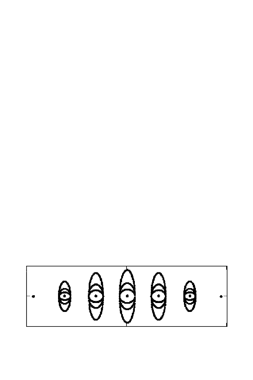
Example 1:
This example demonstrates the impact of changes in the stochastic
model. Figure 4.11 shows a traverse connecting two known stations. Three solutions
Figure 4.11
Impact of changing the stochastic model.