Impact of Sea-Ice Bottom Topography on the Ekman Pumping - Towards an Interdisciplinary Approach in Earth System Science - page 133

that the ice is in motion along x with a constant velocity v ice ¼ 0 : 05 m/s while the

ocean is at rest. We then compute the Ekman pumping with:

w E ¼ z r s

q 0 f ;

ð Þ

4

where

q 0 is the mean density of the sea water,

is the stress at the surface, f is the

s

Coriolis parameter. The stress term is given by:

s

s ¼ q 0 c w j v ice j v ice :

ð 5 Þ

The formulation (Eq. 4 ) of the Ekman vertical velocity is only valid for large
domains in a steady state and our 20 km grid axes may be too small. Nevertheless
we can use such a simpli ed formulation because we are not primarily interested in

quantifying actual Ekman pumping, but we would like to illustrate the importance
of variations in the value of oceanic drag coef

cients alone on the Ekman pumping.
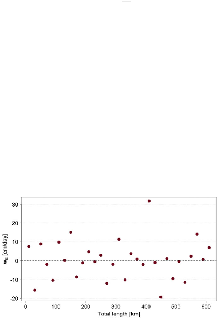
The results of our calculations are shown in Fig. 4 . In this simple experiment there
would not be Ekman pumping if the drag coef cients were constant in the whole

domain. The range of variations of the vertical velocity is between − 20 and 30 cm/
day. Simulated variations in the Ekman vertical velocity based on variations of the
surface stress when no keels are taken into account are shown in Rabe et al. ( 2011 )
(their Fig. 6): Here the range of variations of annual mean vertical velocities over
different regions in the Arctic is between 5 and 3 cm/day. In Rabe et al. ( 2011 ) the

variations in the ocean-surface stress are caused by variations only in the wind

−

eld

and not by variations in the drag coef cients. In our study we see a much higher

variation than in Rabe et al. ( 2011 ) but we stress once more that their result shows
variations averaged over the entire basin while here we focus on local variations.