Geography Reference
In-Depth Information
1
3
A
B
C
AGGLOMERATION
0.9
2.5
A
B
C
0.8
2
0.7
1.5
0.6
EQUIDISTRIBUTION
1
0.5
0.5
0.4
0
100
200
300
400
500
600
0.1
0.2
0.3
0.4
0.5
0.6
0.7
0.8
0.9
x
I
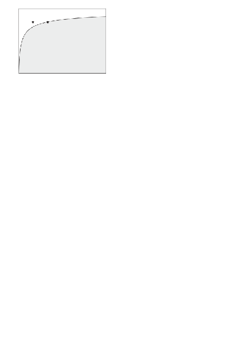
Figure 24
.
3
Entry-exit process for dif erent values of the number of residents I
.
Left panel: A portion of the space (I,
t
) has been divided into the
'agglomeration' area (white) and the 'equidistribution' area (shaded)
according to Proposition 5
.
Right panel: Stationary geographical
distributions computed at the points A, B, and C
.
Other parameters are
a
= 1, μ =0
.
5 and
s
= 4, whereas N is i xed by Assumption 4
1
5
A
B
C
AGGLOMERATION
0.8
4
C
B
A
0.6
3
0.4
2
EQUIDISTRIBUTION
0.2
1
0
0
0.9 0.95
1
1.05 1.1 1.15 1.2 1.25 1.3 1.35 1.4
0.1
0.2
0.3
0.4
0.5
0.6
0.7
0.8
0.9
x
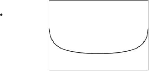
Figure 24
.
4
Entry-exit process for dif erent values of the i xed costs
a.
Left panel: A
portion of the space (
a
,
t
) has been divided into the 'agglomeration' area
(white) and the 'equidistribution' area (shaded) according to Proposition
5
.
Right panel: Stationary geographical distributions computed at the points
A, B, and C
.
Other parameters are I = 400, μ =0
.
5 and
s
= 4 whereas N is
i xed by Assumption 4
points
A
,
B
, and
C
are shown. In both i gures these points have been obtained by keeping
t i xed.
The right panel of Figure 24.3 shows that moving from small to large values of
I
while
keeping t i xed, the long-run distribution changes from bimodal to unimodal. This is
because an increase in the number of residents
I
leads to a decrease in the marginal proi t
b
(see 24.21). In fact, as a result of Assumption 4, the more residents there are, the more
i rms there are and the smaller the contribution of each i rm's locational decision to the
proi ts of other i rms, that is, the smaller the marginal proi t. Changing
I
corresponds to