Capacity Planning - The Practice of Cloud System Administration - page 378

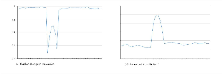
Figure 18.4a shows a sharp drop in correlation corresponding to a change in resource
usage patterns between one software release and the next. The change in correlation in the
graph actually corresponds to a step-change in resource usage patterns from one release
to the next. After the time interval chosen for the rolling correlation measurement elapses,
correlation returns to normal.
Figure 18.4: Change in correlation between MAU and bandwidth
Figure18.4b shows b forthesametimeinterval.Noticethataftertheupgrade b changes
significantly during the time period chosen for the correlation analysis and then becomes
stable again but at a higher value. The large fluctuations in b for the length of the correla-
tion window are due to significant changes in the moving averages from day to day, as the
moving average has both pre- and post-upgrade data. When sufficient time has passed so
thatonlypost-upgradedataisusedinthemovingaverage, b becomesstableandthecorrel-
ation coefficient returns to its previous high levels.
Thevalueof b correspondstotheslopeoftheline,orthemultiplierintheequationlink-
ing the core driver and the usage of the primary resource. When correlation returns to nor-
mal, b is at a higher level. This result indicates that the primary resource will be consumed
more rapidly with this software release than with the previous one. Any marked change in
correlation should trigger a reevaluation of the multiplier b and corresponding resource us-
age predictions.
Forecasting
Forecasting attempts to predict future needs based on current and past measurements. The
most basic forecasting technique is to graph the 90th percentile of the historical usage and
thenfindanequationthatbestfitsthisdata.Youcanthenusethatequationtopredictfuture
usage. Calculating percentiles was discussed in Section 17.5.1 .